分析和优化
介绍
Pine Script™ 是一种基于云的编译语言,旨在高效地重复执行脚本。当用户将 Pine 脚本添加到图表时,它会执行多次,每次执行一次访问数据源中可用的条形图或刻度线,如本手册的执行模型页面中所述 。
Pine Script™ 编译器会自动执行多项内部优化,以适应各种大小的脚本并帮助它们顺利运行。但是,此类优化无法避免脚本执行中的性能瓶颈。因此,程序员需要 分析脚本的运行时性能,并在需要缩短执行时间时找出修改关键代码块和行的方法。
本页介绍如何使用 Pine Profiler分析和监控脚本的运行时和执行情况,并解释了程序员可以修改其代码以 优化运行时性能的一些方法。
松木剖面仪
在深入 优化之前,明智的做法是评估脚本的运行时间并找出 瓶颈,即代码中对整体性能有重大影响的区域。有了这些见解,程序员可以确保专注于优化真正重要的地方,而不是花时间和精力在影响较小的代码上。
输入Pine Profiler,这是一个功能强大的实用程序,可分析脚本中所有重要代码行和块的执行情况,并在 Pine Editor 中的行旁边显示有用的性能信息。通过检查 Profiler 的结果,程序员可以更清楚地了解脚本的整体运行时间、运行时间在其重要代码区域中的分布以及可能需要额外关注和优化的关键部分。
分析脚本
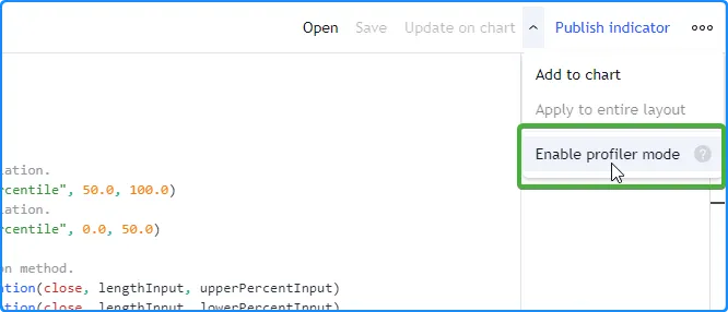
Pine Profiler 可以分析用 Pine Script™ v5 编写的任何可编辑 脚本的运行时性能。要分析脚本,请将其添加到图表中,在 Pine Editor 中打开源代码,然后从右上角“添加到图表/在图表上更新”选项旁边的下拉菜单中选择“启用分析器模式”:
我们将使用下面的脚本作为我们的初始分析示例,该脚本oscillator根据
收盘价与条形图
上百分位数
和下
百分位数lengthInput的平均距离计算自定义值。它包括几种不同类型的
重要代码区域,在分析时,这些代码区域的解释会有所不同
:
//@version=5
indicator("Pine Profiler demo")

//@variable The number of bars in the calculations.
int lengthInput = input.int(100, "Length", 2)
//@variable The percentage for upper percentile calculation.
float upperPercentInput = input.float(75.0, "Upper percentile", 50.0, 100.0)
//@variable The percentage for lower percentile calculation.
float lowerPercentInput = input.float(25.0, "Lower percentile", 0.0, 50.0)

// Calculate percentiles using the linear interpolation method.
float upperPercentile = ta.percentile_linear_interpolation(close, lengthInput, upperPercentInput)
float lowerPercentile = ta.percentile_linear_interpolation(close, lengthInput, lowerPercentInput)

// Declare arrays for upper and lower deviations from the percentiles on the same line.
var upperDistances = array.new<float>(lengthInput), var lowerDistances = array.new<float>(lengthInput)

// Queue distance values through the `upperDistances` and `lowerDistances` arrays based on excessive price deviations.
if math.abs(close - 0.5 * (upperPercentile + lowerPercentile)) > 0.5 * (upperPercentile - lowerPercentile)
    array.push(upperDistances, math.max(close - upperPercentile, 0.0))
    array.shift(upperDistances)
    array.push(lowerDistances, math.max(lowerPercentile - close, 0.0))
    array.shift(lowerDistances)

//@variable The average distance from the `upperDistances` array.
float upperAvg = upperDistances.avg()
//@variable The average distance from the `lowerDistances` array.
float lowerAvg = lowerDistances.avg()
//@variable The ratio of the difference between the `upperAvg` and `lowerAvg` to their sum.
float oscillator = (upperAvg - lowerAvg) / (upperAvg + lowerAvg)
//@variable The color of the plot. A green-based gradient if `oscillator` is positive, a red-based gradient otherwise.
color oscColor = oscillator > 0 ?
     color.from_gradient(oscillator, 0.0, 1.0, color.gray, color.green) :
     color.from_gradient(oscillator, -1.0, 0.0, color.red, color.gray)

// Plot the `oscillator` with the `oscColor`.
plot(oscillator, "Oscillator", oscColor, style = plot.style_area)
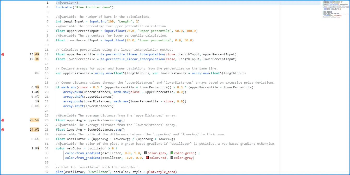
一旦启用,Profiler 会从脚本的重要代码行和块的所有执行中收集信息,然后在 Pine 编辑器内的代码行左侧显示条形图和大致的运行时间百分比:
注意:
- Profiler 跟踪重要代码区域的每次执行,包括实时执行。其信息会随着新执行的发生而不断更新。
- 对于脚本声明语句、类型声明和其他无关紧要的代码行(例如没有实际影响的变量声明、脚本输出不依赖的 未使用代码或编译器在翻译过程中优化的 重复代码) ,分析器结果不会显示。请参阅本节了解更多信息。
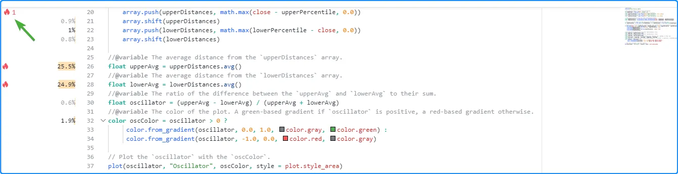
当脚本包含至少四行重要代码时,Profiler 将在性能影响最大的前三个代码区域旁边显示“火焰”图标。如果一个或多个影响最大的代码区域超出了Pine Editor 中可见的行数,则左边距的顶部或底部将显示一个“火焰”图标和一个数字,表示有多少关键行超出了视图。单击图标将垂直滚动编辑器窗口以显示最近的关键行:
将鼠标指针悬停在行旁边的空间上会突出显示已分析的代码,并显示包含其他信息的工具提示,包括所花费的时间和执行次数。每行旁边和相应工具提示中显示的信息取决于所分析的代码区域。以下 部分介绍了 Profiler 分析的不同类型的代码以及如何解释它们的性能结果。
解释分析结果
单行结果
对于包含单行表达式的代码行,Profiler 栏和显示的百分比表示脚本在该行上花费的总运行时间的相对比例。相应的工具提示显示三个字段:
- “行号”字段表示分析的代码行。
- “时间”字段显示代码行的运行时间百分比、该行所花费的运行时间以及脚本的总运行时间。
- “执行”字段显示运行脚本时特定行执行的次数。
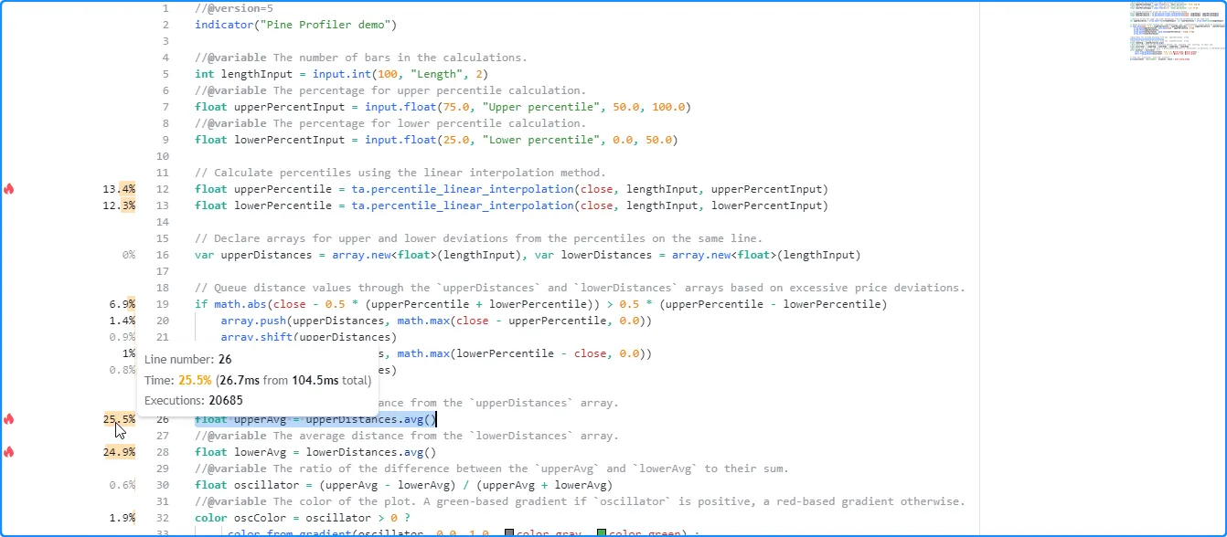
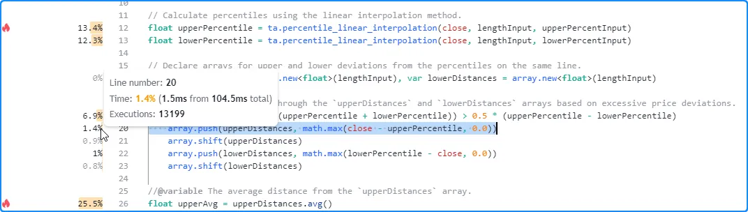
在这里,我们将指针悬停在所分析代码的第 12 行旁边的空间上,以查看其工具提示:
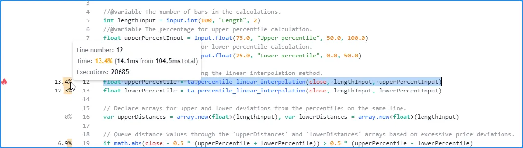
float upperPercentile = ta.percentile_linear_interpolation(close, lengthInput, upperPercentInput)
注意:
- 该行的时间信息代表完成所有执行所花费的时间,而不是单次执行所花费的时间。
- 要估算每次执行的平均时间,请将行的时间除以执行次数。在本例中,工具提示显示第 12 行执行 20,685 次花费了大约 14.1 毫秒,这意味着每次执行的平均时间约为 14.1 毫秒/20685 = 0.0006816534 毫秒(0.6816534 微秒)。
当一行代码由多个用逗号分隔的表达式组成时,工具提示中显示的执行次数表示 每个表达式的总执行次数的总和,显示的时间值表示评估该行所有表达式所花费的总时间。
例如,我们初始示例中的这个全局行包含两个 用逗号分隔的 变量声明。每个都使用var 关键字,这意味着脚本仅在第一个可用条上执行一次。正如我们在该行的 Profiler 工具提示中看到的那样,它计算了两次执行(每个表达式一次),显示的时间值是该行上两个表达式的组合结果:
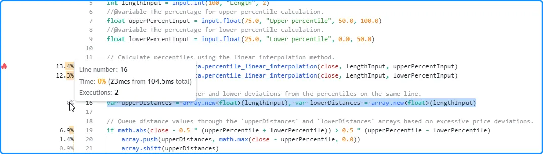
var upperDistances = array.new<float>(lengthInput), var lowerDistances = array.new<float>(lengthInput)
注意:
- 当分析同一行上有多个表达式的脚本时,我们建议将每个表达式移动到单独的行 ,以便在分析时获得更详细的见解,即如果它们可能包含影响更大的计算。
当为了可读性或风格目的而使用 换行时,Profiler 会将换行的所有部分视为 Pine 编辑器中第一行的一部分。
例如,尽管我们初始脚本中的这段代码在 Pine 编辑器中占据了多行,但它仍被视为一行代码,并且 Profiler 工具提示会显示单行结果,其中“行号”字段显示换行所在的编辑器中的第一行:
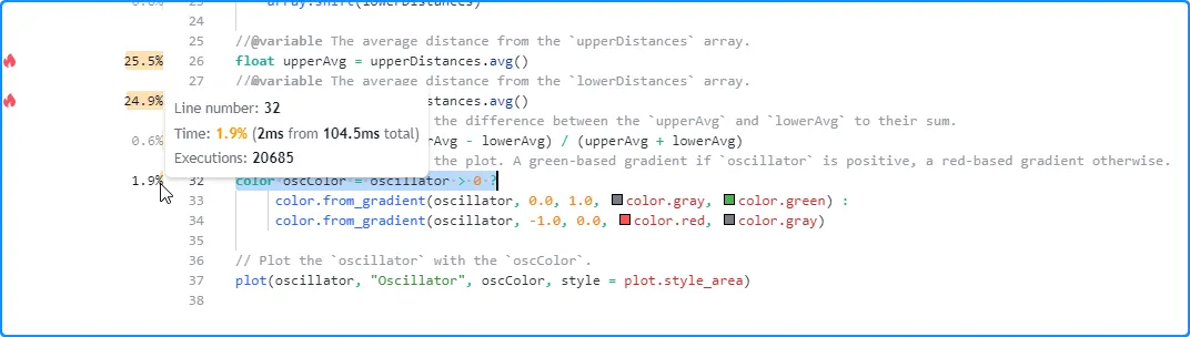
color oscColor = oscillator > 0 ?
     color.from_gradient(oscillator, 0.0, 1.0, color.gray, color.green) :
     color.from_gradient(oscillator, -1.0, 0.0, color.red, color.gray)
代码块结果
对于循环或 条件结构开头的一行,Profiler 栏和百分比表示脚本运行时间在整个代码块(而不仅仅是单行)上所占的相对比例。相应的工具提示显示四个字段:
- “代码块范围”字段表示该结构包含的行范围。
- “时间”字段显示代码块的运行时间百分比、所有块执行所花费的时间以及脚本的总运行时间。
- “行时间”字段显示块的初始行的运行时间百分比、在该行上花费的时间以及脚本的总运行时间。对于 switch 块或 带有else if语句的if 块,其解释有所不同,因为这些值表示在所有 结构的条件语句 上花费的总时间。有关更多信息,请参阅下文。
- “执行”字段显示运行脚本时代码块执行的次数。
在这里,我们将鼠标悬停在初始脚本中第 19 行旁边的空间上,这是一个简单的 if 结构的开头,没有 else if 语句。如下所示,工具提示显示了整个代码块和当前行的性能信息:
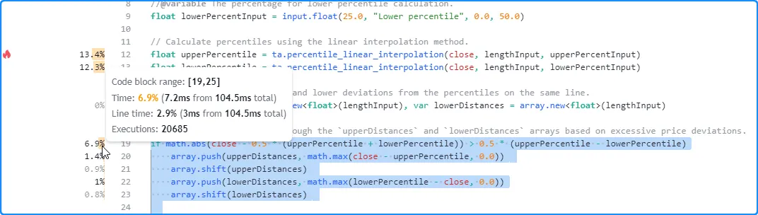
if math.abs(close - 0.5 * (upperPercentile + lowerPercentile)) > 0.5 * (upperPercentile - lowerPercentile)
    array.push(upperDistances, math.max(close - upperPercentile, 0.0))
    array.shift(upperDistances)
    array.push(lowerDistances, math.max(lowerPercentile - close, 0.0))
    array.shift(lowerDistances)
注意:
- “时间”字段显示,对该结构进行 20,685 次求值总共花费了 7.2 毫秒。
- “行时间”字段表示 此 if结构第一行所花费的运行时间 约为三毫秒。
用户还可以检查代码块范围内的行和嵌套块的结果,以获得更细致的性能洞察。在这里,我们将鼠标悬停在代码块内第 20 行旁边的空间上,以查看其 单行结果:
注意:
- 显示的执行次数小于整个代码块的结果,因为控制此行执行的条件并非始终返回。循环
true内的代码则相反,因为每次执行循环语句都会触发 多次执行循环的局部块。
在分析 switch 结构或 包含else if语句的if结构时 ,“行时间”字段将显示执行 结构的所有条件表达式(而不仅仅是块的第一行)所花费的时间。代码块范围内的行的结果将显示每个本地块的运行时间和执行情况。由于 Profiler 的计算和显示限制,这种格式对于这些结构是必需的。 有关更多信息,请参阅本节。
例如, 此脚本中switch结构的“行时间”表示评估其主体内所有四个条件语句 所花费的时间 ,因为 Profiler无法单独跟踪它们。代码块范围内每行的结果代表每个本地块的性能信息:
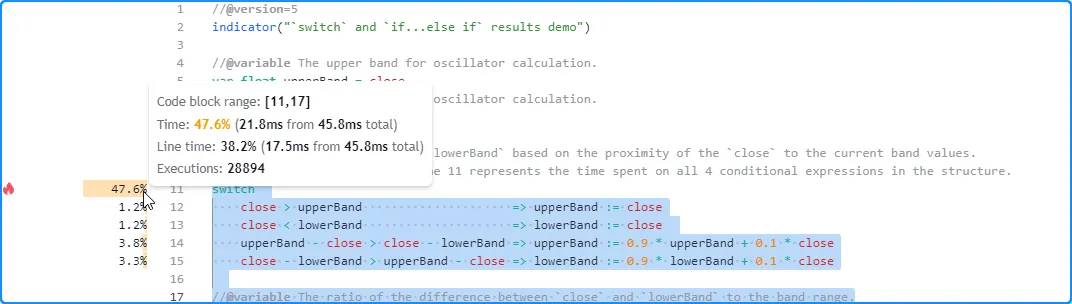
//@version=5
indicator("`switch` and `if...else if` results demo")

//@variable The upper band for oscillator calculation.
var float upperBand = close
//@variable The lower band for oscillator calculation.
var float lowerBand = close

// Update the `upperBand` and `lowerBand` based on the proximity of the `close` to the current band values.
// The "Line time" field on line 11 represents the time spent on all 4 conditional expressions in the structure.
switch
    close > upperBand                     => upperBand := close
    close < lowerBand                     => lowerBand := close
    upperBand - close > close - lowerBand => upperBand := 0.9 * upperBand + 0.1 * close
    close - lowerBand > upperBand - close => lowerBand := 0.9 * lowerBand + 0.1 * close

//@variable The ratio of the difference between `close` and `lowerBand` to the band range.
float oscillator = 100.0 * (close - lowerBand) / (upperBand - lowerBand)

// Plot the `oscillator` as columns with a dynamic color.
plot(
     oscillator, "Oscillator", oscillator > 50.0 ? color.teal : color.maroon,
     style = plot.style_columns, histbase = 50.0
 )
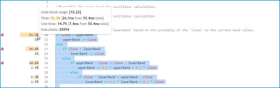
当此类结构中的条件逻辑涉及大量计算时,程序员可能需要针对每个计算条件提供更详细的性能信息。实现此分析的有效方法是使用嵌套 if块,而不是更紧凑的 switch 或if…else if 结构。例如,而不是:
switch
    <expression1> => <localBlock1>
    <expression2> => <localBlock2>
    =>               <localBlock3>
或者:
if <expression1>
    <localBlock1>
else if <expression2>
    <localBlock2>
else
    <localBlock3>
可以使用嵌套的 if块进行更深入的分析,同时保持相同的逻辑流程:
if <expression1>
    <localBlock1>
else
    if <expression2>
        <localBlock2>
    else
        <localBlock3>
下面,我们将前面的 switch 示例更改为等效的嵌套 if 结构。现在,我们可以分别查看条件模式每个重要部分的运行时和执行情况:
//@version=5
indicator("`switch` and `if...else if` results demo")

//@variable The upper band for oscillator calculation.
var float upperBand = close
//@variable The lower band for oscillator calculation.
var float lowerBand = close

// Update the `upperBand` and `lowerBand` based on the proximity of the `close` to the current band values.
if close > upperBand
    upperBand := close
else
    if close < lowerBand
        lowerBand := close
    else
        if upperBand - close > close - lowerBand
            upperBand := 0.9 * upperBand + 0.1 * close
        else
            if close - lowerBand > upperBand - close
                lowerBand := 0.9 * lowerBand + 0.1 * close

//@variable The ratio of the difference between `close` and `lowerBand` to the band range.
float oscillator = 100.0 * (close - lowerBand) / (upperBand - lowerBand)

// Plot the `oscillator` as columns with a dynamic color.
plot(
     oscillator, "Oscillator", oscillator > 50.0 ? color.teal : color.maroon,
     style = plot.style_columns, histbase = 50.0
 )
注意:
用户定义函数调用
用户定义函数和 方法 是由用户编写的函数。它们封装了脚本可能多次执行的代码序列。用户经常编写函数和方法以提高代码的模块化、可重用性和可维护性。
函数内缩进的代码行表示其局部作用域,即每次脚本调用时执行的序列。与脚本全局作用域中的代码(脚本每次执行时都会评估一次)不同,函数内的代码在每次脚本执行时可能会激活零次、一次或多次,具体取决于触发调用的条件、发生的调用次数以及函数的逻辑。
在解释 Profiler 结果时,考虑这一区别至关重要。当分析的代码包含 用户定义的函数或 方法 调用时:
- 每个函数调用的结果反映了分配给它的运行时间以及脚本激活该特定调用的总次数。
- 函数范围内所有本地代码的时间和执行信息反映了对该函数的所有调用的综合结果。
此示例包含一个用户定义similarity()函数,用于估算两个系列的相似度,脚本每次执行时仅从全局范围调用
一次该函数。在本例中,Profiler 对函数主体内代码的结果与该特定调用相对应:
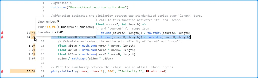
//@version=5
indicator("User-defined function calls demo")

//@function Estimates the similarity between two standardized series over `length` bars.
//          Each individual call to this function activates its local scope.
similarity(float sourceA, float sourceB, int length) =>
    // Standardize `sourceA` and `sourceB` for comparison.
    float normA = (sourceA - ta.sma(sourceA, length)) / ta.stdev(sourceA, length)
    float normB = (sourceB - ta.sma(sourceB, length)) / ta.stdev(sourceB, length)
    // Calculate and return the estimated similarity of `normA` and `normB`.
    float abSum = math.sum(normA * normB, length)
    float a2Sum = math.sum(normA * normA, length)
    float b2Sum = math.sum(normB * normB, length)
    abSum / math.sqrt(a2Sum * b2Sum)

// Plot the similarity between the `close` and an offset `close` series.
plot(similarity(close, close[1], 100), "Similarity 1", color.red)
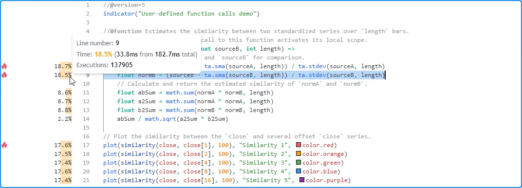
让我们增加脚本每次执行时调用该函数的次数。在这里,我们将脚本更改为调用用户 定义函数 五次:
//@version=5
indicator("User-defined function calls demo")

//@function Estimates the similarity between two standardized series over `length` bars.
//          Each individual call to this function activates its local scope.
similarity(float sourceA, float sourceB, int length) =>
    // Standardize `sourceA` and `sourceB` for comparison.
    float normA = (sourceA - ta.sma(sourceA, length)) / ta.stdev(sourceA, length)
    float normB = (sourceB - ta.sma(sourceB, length)) / ta.stdev(sourceB, length)
    // Calculate and return the estimated similarity of `normA` and `normB`.
    float abSum = math.sum(normA * normB, length)
    float a2Sum = math.sum(normA * normA, length)
    float b2Sum = math.sum(normB * normB, length)
    abSum / math.sqrt(a2Sum * b2Sum)

// Plot the similarity between the `close` and several offset `close` series.
plot(similarity(close, close[1], 100), "Similarity 1", color.red)
plot(similarity(close, close[2], 100), "Similarity 2", color.orange)
plot(similarity(close, close[4], 100), "Similarity 3", color.green)
plot(similarity(close, close[8], 100), "Similarity 4", color.blue)
plot(similarity(close, close[16], 100), "Similarity 5", color.purple)
在这种情况下,本地代码结果不再对应于每个脚本执行的单个
评估。相反,它们代表所有五次调用
的本地代码的综合运行时间和执行情况。如下所示,在相同数据上运行此版本的脚本后的结果显示本地代码执行了 137,905 次,是
脚本仅包含一个函数调用时的五倍
:similarity()
请求其他上下文时
Pine 脚本可以通过调用函数系列或在
indicator()声明语句中指定替代方案来从其他上下文请求数据,即与图表数据使用的不同的符号、时间范围或数据修改
。request.*()timeframe
当脚本从另一个上下文请求数据时,它会评估该上下文中所有必需的范围和计算,如 其他时间范围和数据页面中所述。此行为会影响脚本代码区域的运行时间及其执行的次数。
任何代码行或 块的 Profiler 信息 代表在所有必要上下文中执行代码的结果,这些结果可能包含也可能不包含图表的数据。Pine Script™ 根据脚本的数据请求和输出所需的计算来确定在哪些上下文中执行代码。
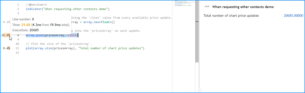
让我们看一个简单的例子。这个初始脚本仅使用图表的数据进行计算。它使用varippricesArray关键字声明一个变量
,这意味着
分配给它的数组
在数据历史记录和所有可用的实时刻度中保持不变。每次执行时,脚本都会调用
array.push()
将新的
收盘
价
推送到数组中,并绘制数组的大小。
在日内图表的所有条形图上对脚本进行分析后,我们看到元素的数量与pricesArrayProfiler 在第 8 行显示的
array.push()调用的执行次数相对应
:
//@version=5
indicator("When requesting other contexts demo")

//@variable An array containing the `close` value from every available price update.
varip array<float> pricesArray = array.new<float>()

// Push a new `close` value into the `pricesArray` on each update.
array.push(pricesArray, close)

// Plot the size of the `pricesArray`.
plot(array.size(pricesArray), "Total number of chart price updates")
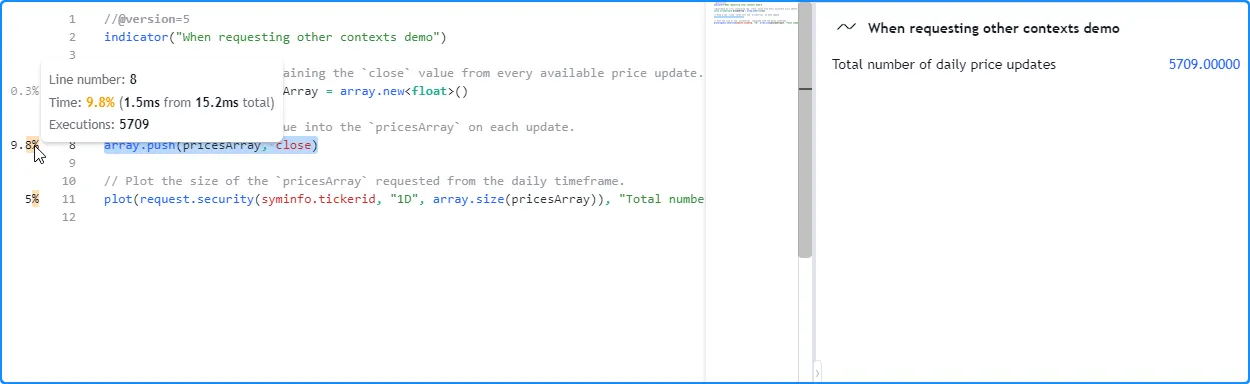
pricesArray现在,让我们尝试从另一个上下文评估大小,而不是使用图表的数据。下面,我们添加了一个
request.security()
调用,以
array.size(pricesArray)
作为其expression参数,以检索在“1D”时间范围内计算的值并绘制该结果。
在这种情况下,Profiler 在第 8 行显示的执行次数仍然与 中的元素数量相对应。但是,由于脚本在计算中
pricesArray不需要图表的数据,因此执行的次数并不相同。它只需要初始化数组
并对所有请求的每日数据
评估
array.push(),其价格更新次数与我们当前的日内图表不同:
//@version=5
indicator("When requesting other contexts demo")

//@variable An array containing the `close` value from every available price update.
varip array<float> pricesArray = array.new<float>()

// Push a new `close` value into the `pricesArray` on each update.
array.push(pricesArray, close)

// Plot the size of the `pricesArray` requested from the daily timeframe.
plot(request.security(syminfo.tickerid, "1D", array.size(pricesArray)), "Total number of daily price updates")
注意:
- 本例中请求的 EOD 数据的数据点比我们的日内图表少,因此 在这种情况下 array.push()调用需要的执行次数较少。但是,EOD 源没有历史记录限制,这意味着请求的 HTF 数据也可能比用户的图表跨越更多的条形图,具体取决于时间范围、数据提供商和用户的计划。
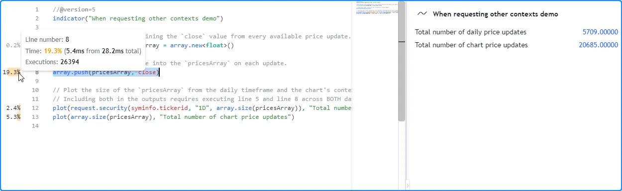
如果此脚本除了请求的每日值之外还直接绘制 array.size() 值,则需要创建两个 数组(每个上下文一个),并 跨图表数据和每日时间范围的数据执行 array.push()。因此,第 5 行上的声明将执行两次,第 8 行上的结果将反映从评估两个独立数据 集上的array.push()调用所累积的时间和执行次数 :
//@version=5
indicator("When requesting other contexts demo")

//@variable An array containing the `close` value from every available price update.
varip array<float> pricesArray = array.new<float>()

// Push a new `close` value into the `pricesArray` on each update.
array.push(pricesArray, close)

// Plot the size of the `pricesArray` from the daily timeframe and the chart's context.
// Including both in the outputs requires executing line 5 and line 8 across BOTH datasets.
plot(request.security(syminfo.tickerid, "1D", array.size(pricesArray)), "Total number of daily price updates")
plot(array.size(pricesArray), "Total number of chart price updates")
需要注意的是,当脚本调用包含
本地作用域内调用的
用户定义函数或
方法时,脚本的翻译形式会提取作用域外的调用,并将它们依赖的表达式封装在单独的函数中。脚本执行时,会先评估所需的
调用,然后将请求的数据
传递给用户定义函数的
修改形式。request.*()request.*()request.*()
由于翻译后的脚本
在评估其本地范围内未请求的计算之前会单独执行用户定义函数的数据请求,因此,Profiler 对包含对该函数的调用的行的结果将不包括在其调用或所需表达式上花费的时间。request.*()
例如,以下脚本包含一个用户定义
getCompositeAvg()函数,该函数带有
request.security()
调用,该调用请求
来自指定 的
10 个
ta.wma()调用的math.avg ()
,这些调用具有不同的参数。该脚本使用该函数使用Heikin Ashi股票代码 ID请求平均结果
:lengthsymbol
//@version=5
indicator("User-defined functions with `request.*()` calls demo", overlay = true)

int multInput = input.int(10, "Length multiplier", 1)

string tickerID = ticker.heikinashi(syminfo.tickerid)

getCompositeAvg(string symbol, int lengthMult) =>
    request.security(
         symbol, timeframe.period, math.avg(
             ta.wma(close, lengthMult), ta.wma(close, 2 * lengthMult), ta.wma(close, 3 * lengthMult),
             ta.wma(close, 4 * lengthMult), ta.wma(close, 5 * lengthMult), ta.wma(close, 6 * lengthMult),
             ta.wma(close, 7 * lengthMult), ta.wma(close, 8 * lengthMult), ta.wma(close, 9 * lengthMult),
             ta.wma(close, 10 * lengthMult)
         )
     )

plot(getCompositeAvg(tickerID, multInput), "Composite average", linewidth = 3)
对脚本进行分析后,用户可能会惊讶地发现函数主体内部显示的运行时结果大大超过单次 调用显示的结果getCompositeAvg():
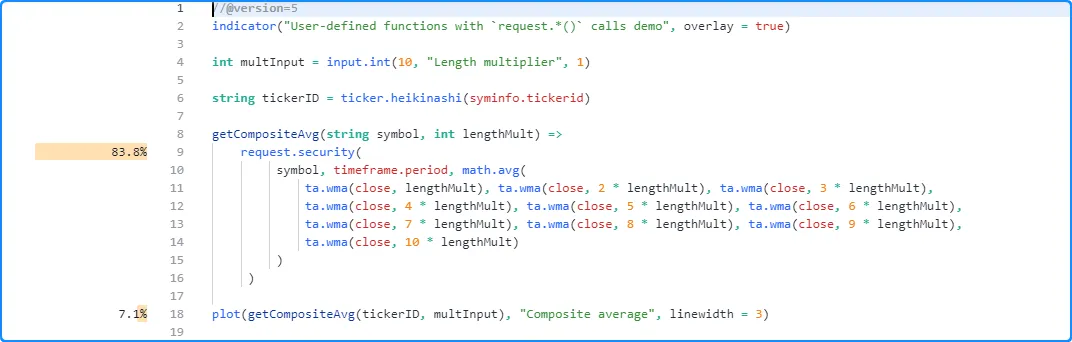
结果之所以这样显示,是因为翻译后的脚本包含内部修改,将request.security () 调用及其表达式移到了函数范围之外,并且在这种情况下,Profiler 除了将这些计算的结果显示在request.security()行旁边之外,没有其他方法可以表示这些计算的结果 。下面的代码大致说明了翻译后的脚本的样子:
//@version=5
indicator("User-defined functions with `request.*()` calls demo", overlay = true)

int multInput = input.int(10, "Length multiplier")

string tickerID = ticker.heikinashi(syminfo.tickerid)

secExpr(int lengthMult)=>
    math.avg(
         ta.wma(close, lengthMult), ta.wma(close, 2 * lengthMult), ta.wma(close, 3 * lengthMult),
         ta.wma(close, 4 * lengthMult), ta.wma(close, 5 * lengthMult), ta.wma(close, 6 * lengthMult),
         ta.wma(close, 7 * lengthMult), ta.wma(close, 8 * lengthMult), ta.wma(close, 9 * lengthMult),
         ta.wma(close, 10 * lengthMult)
     )

float sec = request.security(tickerID, timeframe.period, secExpr(multInput))

getCompositeAvg(float s) =>
    s

plot(getCompositeAvg(sec), "Composite average", linewidth = 3)
注意:
- 该
secExpr()代码代表request.security() 用来计算请求上下文中所需表达式的 单独函数。 - request.security
()
调用发生在函数之外的
外部作用域中
getCompositeAvg()。 - 翻译大大减少了 的本地代码
getCompositeAvg()。它现在仅返回传递给它的值,因为函数所需的所有计算都发生 在其范围之外。由于这种减少,函数调用的性能结果将不会反映出数据请求所需计算所花费的任何时间。
不重要、未使用和冗余的代码
在检查分析脚本的结果时,务必要了解脚本中
并非所有代码都会影响运行时性能。有些代码不会直接影响性能,例如脚本的声明语句和类型
声明。其他具有不重要表达式的代码区域(例如大多数input.*()调用、变量引用或
没有重要计算的变量声明)对脚本的运行时几乎没有影响
。因此,Profiler 不会显示这些类型代码的性能结果。
此外,Pine 脚本不会执行其 输出(绘图、 图纸、 日志等)不依赖的代码区域,因为编译器会在翻译过程中自动删除它们。由于未使用的代码区域对脚本的性能没有任何影响,因此 Profiler 不会显示它们的任何结果。
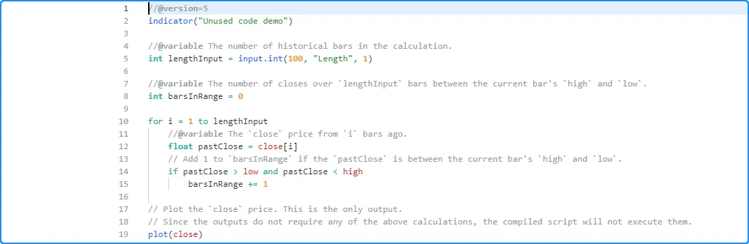
以下示例包含一个barsInRange变量和一个
for循环,该循环将
当前
最高价
和最低价之间的每个历史收盘价加 1 到变量的值
。但是,脚本不会在其输出中使用这些计算,因为它只
绘制收盘价
。因此,脚本的编译形式会丢弃未使用的代码,只考虑
plot (close)
调用。lengthInput
Profiler 不会显示此脚本的任何结果,因为它不执行任何重要的计算:
//@version=5
indicator("Unused code demo")

//@variable The number of historical bars in the calculation.
int lengthInput = input.int(100, "Length", 1)

//@variable The number of closes over `lengthInput` bars between the current bar's `high` and `low`.
int barsInRange = 0

for i = 1 to lengthInput
    //@variable The `close` price from `i` bars ago.
    float pastClose = close[i]
    // Add 1 to `barsInRange` if the `pastClose` is between the current bar's `high` and `low`.
    if pastClose > low and pastClose < high
        barsInRange += 1

// Plot the `close` price. This is the only output.
// Since the outputs do not require any of the above calculations, the compiled script will not execute them.
plot(close)
注意:
- 虽然该脚本不使用 第 5 行的input.int() 并丢弃所有相关计算,但“Length”输入仍会出现在脚本的设置中,因为编译器不会完全删除未使用的 输入。
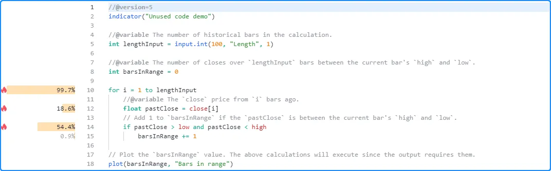
如果我们将脚本改为绘制barsInRange值,则声明的变量和
for循环不再未被使用,因为输出依赖于它们,并且 Profiler 现在将显示该代码的性能信息:
//@version=5
indicator("Unused code demo")

//@variable The number of historical bars in the calculation.
int lengthInput = input.int(100, "Length", 1)

//@variable The number of closes over `lengthInput` bars between the current bar's `high` and `low`.
int barsInRange = 0

for i = 1 to lengthInput
    //@variable The `close` price from `i` bars ago.
    float pastClose = close[i]
    // Add 1 to `barsInRange` if the `pastClose` is between the current bar's `high` and `low`.
    if pastClose > low and pastClose < high
        barsInRange += 1

// Plot the `barsInRange` value. The above calculations will execute since the output requires them.
plot(barsInRange, "Bars in range")
注意:
- Profiler 不会显示
lengthInput第 5 行的声明或barsInRange第 8 行的声明的性能信息,因为这些行上的表达式不会影响脚本的性能。
如果可能,编译器还会简化脚本中的某些冗余代码实例 ,例如具有相同 基本类型 值的某些相同表达式形式。这种优化允许编译后的脚本在第一次出现时仅执行一次此类计算,并对输出所依赖的每个重复实例重用计算结果。
如果脚本包含重复代码并且编译器对其进行了简化,则 Profiler 将仅显示该代码第一次出现的结果,因为这是脚本唯一需要计算的时候。
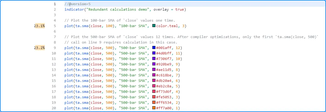
例如,此脚本包含绘制ta.sma(close, 100)值的代码行 和绘制ta.sma(close, 500) 值的代码行:
//@version=5
indicator("Redundant calculations demo", overlay = true)

// Plot the 100-bar SMA of `close` values one time.
plot(ta.sma(close, 100), "100-bar SMA", color.teal, 3)

// Plot the 500-bar SMA of `close` values 12 times. After compiler optimizations, only the first `ta.sma(close, 500)`
// call on line 9 requires calculation in this case.
plot(ta.sma(close, 500), "500-bar SMA", #001aff, 12)
plot(ta.sma(close, 500), "500-bar SMA", #4d0bff, 11)
plot(ta.sma(close, 500), "500-bar SMA", #7306f7, 10)
plot(ta.sma(close, 500), "500-bar SMA", #920be9, 9)
plot(ta.sma(close, 500), "500-bar SMA", #ae11d5, 8)
plot(ta.sma(close, 500), "500-bar SMA", #c618be, 7)
plot(ta.sma(close, 500), "500-bar SMA", #db20a4, 6)
plot(ta.sma(close, 500), "500-bar SMA", #eb2c8a, 5)
plot(ta.sma(close, 500), "500-bar SMA", #f73d6f, 4)
plot(ta.sma(close, 500), "500-bar SMA", #fe5053, 3)
plot(ta.sma(close, 500), "500-bar SMA", #ff6534, 2)
plot(ta.sma(close, 500), "500-bar SMA", #ff7a00, 1)
由于最后 12 行都包含相同的 ta.sma() 调用,编译器可以自动简化脚本,以便每次执行只需要评估一次ta.sma(close, 500), 而不是重复计算 11 次。
如下所示,Profiler 仅显示第 5 行和第 9 行的结果。这些是代码中唯一需要大量计算的部分,因为 在这种情况下,第 10-20 行的ta.sma() 调用是多余的:
另一种重复代码优化发生在脚本包含两个或多个 具有相同编译形式的用户定义函数或 方法时 。在这种情况下,编译器通过删除冗余函数来简化脚本,并且脚本会将对冗余函数的所有调用视为对第一个 定义版本的调用。因此,Profiler 将仅显示第一个函数的本地代码性能结果,因为丢弃的“克隆”永远不会执行。
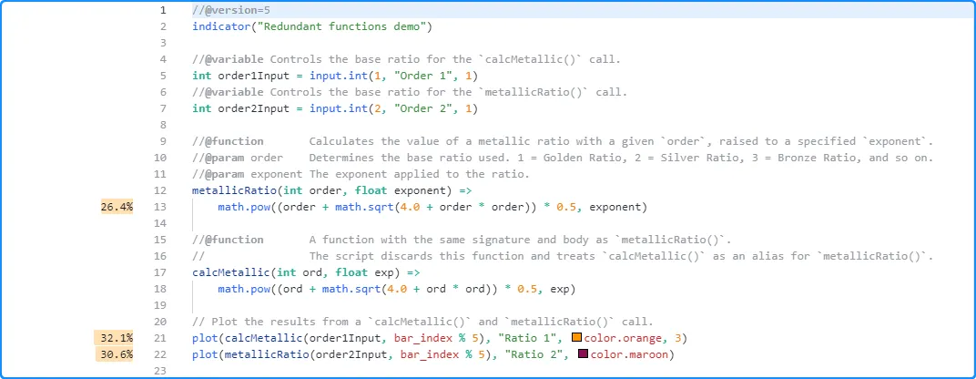
例如,下面的脚本包含两个
用户定义函数,metallicRatio()和calcMetallic(),用于计算
给定阶的指定指数的金属比:
//@version=5
indicator("Redundant functions demo")

//@variable Controls the base ratio for the `calcMetallic()` call.
int order1Input = input.int(1, "Order 1", 1)
//@variable Controls the base ratio for the `metallicRatio()` call.
int order2Input = input.int(2, "Order 2", 1)

//@function       Calculates the value of a metallic ratio with a given `order`, raised to a specified `exponent`.
//@param order    Determines the base ratio used. 1 = Golden Ratio, 2 = Silver Ratio, 3 = Bronze Ratio, and so on.
//@param exponent The exponent applied to the ratio.
metallicRatio(int order, float exponent) =>
    math.pow((order + math.sqrt(4.0 + order * order)) * 0.5, exponent)

//@function       A function with the same signature and body as `metallicRatio()`.
//                The script discards this function and treats `calcMetallic()` as an alias for `metallicRatio()`.
calcMetallic(int ord, float exp) =>
    math.pow((ord + math.sqrt(4.0 + ord * ord)) * 0.5, exp)

// Plot the results from a `calcMetallic()` and `metallicRatio()` call.
plot(calcMetallic(order1Input, bar_index % 5), "Ratio 1", color.orange, 3)
plot(metallicRatio(order2Input, bar_index % 5), "Ratio 2", color.maroon)
尽管函数和参数名称不同,但这两个函数在其他方面是相同的,编译器在翻译脚本时会检测到这一点。在这种情况下,它会丢弃冗余
calcMetallic()函数,并且编译后的脚本会将该
calcMetallic()调用视为metallicRatio()调用。
正如我们在这里看到的,Profiler 显示了第 21 行和第 22 行的
calcMetallic()和metallicRatio()调用的性能信息,但它没有显示第 18 行函数本地代码的任何结果。calcMetallic()
相反,Profiler 在函数内第 13 行的信息反映了两个函数调用metallicRatio()的本地代码结果:
了解 Profiler 的内部工作原理
Pine Profiler 使用专门的 内部函数包装所有必要的代码区域,以跟踪和收集脚本执行过程中所需的信息。然后,它将信息传递给其他计算,这些计算会在 Pine Editor 中组织和显示性能结果。本节让用户了解 Profiler 如何应用内部函数包装 Pine 代码并收集性能数据。
Profiler使用两个主要的内部(非 Pine)函数包装重要代码,以方便运行时分析。第一个函数检索脚本执行过程中特定点的当前系统时间,第二个函数将累计运行时间和执行数据映射到特定代码区域。我们在本说明中分别将这些函数表示为System.timeNow()和registerPerf()。
当 Profiler 检测到需要分析的代码时,它会
System.timeNow()在代码上方添加,以获取执行前的初始时间。然后,它会registerPerf()在代码下方添加,以映射和累积已用时间和执行次数。每次调用时添加的已用时间registerPerf()是执行后的System.timeNow()值
减去执行前的值。
以下伪代码概述了单行代码的这个过程
,其中_startX表示该行的开始时间lineX:
long _startX = System.timeNow()
<code_line_to_analyze>
registerPerf(System.timeNow() - _startX, lineX)
代码块的过程类似
。不同之处在于registerPerf()调用将数据映射到一系列行而不是单行。这里,lineX
表示代码块中的第一lineY行,表示块的最后一行:
long _startX = System.timeNow()
<code_block_to_analyze>
registerPerf(System.timeNow() - _startX, lineX, lineY)
注意:
- 在上面的代码片段中,、
long和System.timeNow()代表registerPerf()内部代码,而不是Pine Script™ 代码。
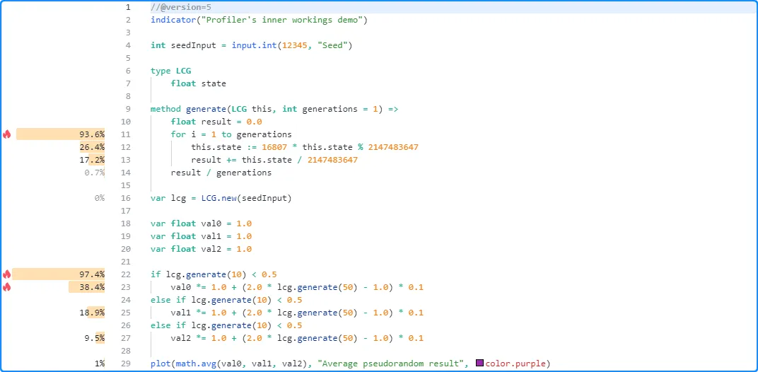
现在让我们看看 Profiler 如何包装完整的脚本及其所有重要代码。我们将从这个脚本开始,它计算三个伪随机序列并显示它们的 平均 结果。该脚本利用用户定义类型的 对象来存储伪随机状态,利用一种 方法 来计算新值并更新状态,以及利用if…else if 结构根据生成的值更新每个序列:
//@version=5
indicator("Profiler's inner workings demo")

int seedInput = input.int(12345, "Seed")

type LCG
    float state

method generate(LCG this, int generations = 1) =>
    float result = 0.0
    for i = 1 to generations
        this.state := 16807 * this.state % 2147483647
        result += this.state / 2147483647
    result / generations

var lcg = LCG.new(seedInput)

var float val0 = 1.0
var float val1 = 1.0
var float val2 = 1.0

if lcg.generate(10) < 0.5
    val0 *= 1.0 + (2.0 * lcg.generate(50) - 1.0) * 0.1
else if lcg.generate(10) < 0.5
    val1 *= 1.0 + (2.0 * lcg.generate(50) - 1.0) * 0.1
else if lcg.generate(10) < 0.5
    val2 *= 1.0 + (2.0 * lcg.generate(50) - 1.0) * 0.1

plot(math.avg(val0, val1, val2), "Average pseudorandom result", color.purple)
Profiler 将使用 上述内部函数包装整个脚本和所有必要的代码区域(不包括任何不重要、未使用或冗余的代码),以收集性能数据。下面的伪代码演示了此过程如何应用于上述脚本:
long _startMain = System.timeNow() // Start time for the script's overall execution.

// <Additional internal code executes here>

//@version=5
indicator("Profiler's inner workings demo") // Declaration statements do not require profiling.

int seedInput = input.int(12345, "Seed") // Variable declaration without significant calculation.

type LCG        // Type declarations do not require profiling.
    float state

method generate(LCG this, int generations = 1) => // Function signature does not affect runtime.
    float result = 0.0 // Variable declaration without significant calculation.

    long _start11 = System.timeNow() // Start time for the loop block that begins on line 11.
    for i = 1 to generations // Loop header calculations are not independently wrapped.

        long _start12 = System.timeNow() // Start time for line 12.
        this.state := 16807 * this.state % 2147483647
        registerPerf(System.timeNow() - _start12, line12) // Register performance info for line 12.

        long _start13 = System.timeNow() // Start time for line 13.
        result += this.state / 2147483647
        registerPerf(System.timeNow() - _start13, line13) // Register performance info for line 13.

    registerPerf(System.timeNow() - _start11, line11, line13) // Register performance info for the block (line 11 - 13).

    long _start14 = System.timeNow() // Start time for line 14.
    result / generations
    registerPerf(System.timeNow() - _start14, line14) // Register performance info for line 14.

long _start16 = System.timeNow() // Start time for line 16.
var lcg = LCG.new(seedInput)
registerPerf(System.timeNow() - _start16, line16) // Register performance info for line 16.

var float val0 = 1.0 // Variable declarations without significant calculations.
var float val1 = 1.0
var float val2 = 1.0

long _start22 = System.timeNow() // Start time for the `if` block that begins on line 22.
if lcg.generate(10) < 0.5 // `if` statement is not independently wrapped.

    long _start23 = System.timeNow() // Start time for line 23.
    val0 *= 1.0 + (2.0 * lcg.generate(50) - 1.0) * 0.1
    registerPerf(System.timeNow() - _start23, line23) // Register performance info for line 23.

else if lcg.generate(10) < 0.5 // `else if` statement is not independently wrapped.

    long _start25 = System.timeNow() // Start time for line 25.
    val1 *= 1.0 + (2.0 * lcg.generate(50) - 1.0) * 0.1
    registerPerf(System.timeNow() - _start25, line25) // Register performance info for line 25.

else if lcg.generate(10) < 0.5 // `else if` statement is not independently wrapped.

    long _start27 = System.timeNow() // Start time for line 27.
    val2 *= 1.0 + (2.0 * lcg.generate(50) - 1.0) * 0.1
    registerPerf(System.timeNow() - _start27, line27) // Register performance info for line 27.

registerPerf(System.timeNow() - _start22, line22, line28) // Register performance info for the block (line 22 - 28).

long _start29 = System.timeNow() // Start time for line 29.
plot(math.avg(val0, val1, val2), "Average pseudorandom result", color.purple)
registerPerf(System.timeNow() - _start29, line29) // Register performance info for line 29.

// <Additional internal code executes here>

registerPerf(System.timeNow() - _startMain, total) // Register the script's overall performance info.
注意:
- 此示例是伪代码,提供了 Profiler 用于收集性能数据的内部计算的基本概述。将此示例保存在 Pine Editor 中将导致编译错误,因为
long、System.timeNow()和registerPerf()不代表Pine Script™ 代码。 - Profiler 封装脚本时使用的这些内部计算需要额外的计算资源,这就是脚本在分析时运行时间增加的原因。程序员应始终将结果解释为估计值 ,因为它们反映了脚本在包含额外计算的情况下的性能。
运行包装的脚本收集性能数据后, 额外的内部计算会组织结果并在 Pine 编辑器内显示相关信息:
代码块的 “行时间”计算也发生在此阶段,因为 Profiler 无法单独包装循环头或if或 switch 结构 中的条件语句 。此字段的值表示块的总时间与其本地代码时间总和之间的 差值,这就是为什么switch 块或 带有else if表达式的if块的“行时间”值表示结构的所有条件语句 所花费的时间,而不仅仅是块的初始代码行。如果程序员需要此类块中每个条件表达式的更详细信息,他们可以将逻辑重新组织为 嵌套的if 结构,如此处 所述。
跨配置分析
当代码的时间复杂度不是恒定的或其执行模式随其输入、函数参数或可用数据而变化时,通常明智的做法是跨不同的配置和数据馈送对代码进行分析,以便更全面地了解其总体性能。
例如,这个简单的脚本使用
for循环来计算当前收盘
价与lengthInput之前价格之间的平方差之和
,然后
在每个柱状图上绘制该和的平方根lengthInput。在这种情况下,直接影响计算的运行时间,因为它决定了循环执行其本地代码的次数:
//@version=5
indicator("Profiling across configurations demo")
//@variable The number of previous bars in the calculation. Directly affects the number of loop iterations.
int lengthInput = input.int(25, "Length", 1)
//@variable The sum of squared distances from the current `close` to `lengthInput` past `close` values.
float total = 0.0
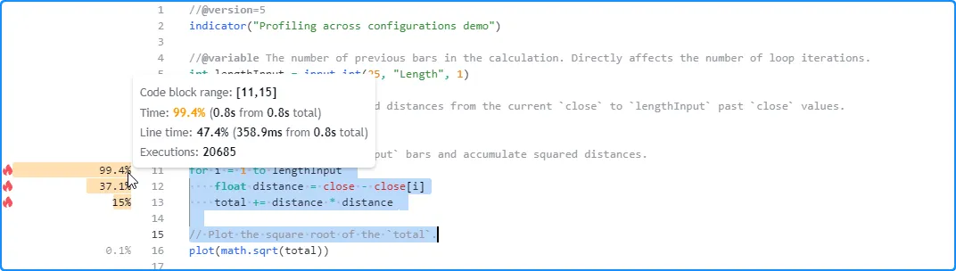
// Look back across `lengthInput` bars and accumulate squared distances.
for i = 1 to lengthInput
float distance = close - close[i]
total += distance * distance
// Plot the square root of the `total`.
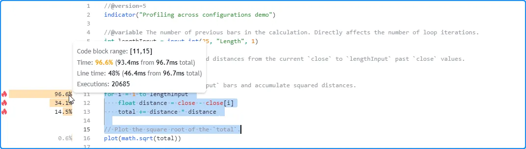
plot(math.sqrt(total))
让我们尝试使用不同的lengthInput值来分析此脚本。首先,我们将使用默认值 25。Profiler 对此次特定运行的结果显示,该脚本在约 96.7 毫秒内完成了 20,685 次执行:
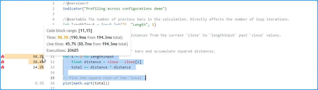
在这里,我们在脚本的设置中将输入的值增加到 50。本次运行的结果显示,脚本的总运行时间为 194.3 毫秒,接近上次运行时间的两倍:
在下一次运行中,我们将输入的值更改为 200。这一次,Profiler 的结果显示脚本在大约 0.8 秒内完成所有执行,大约是上次运行时间的四倍:
从这些观察中我们可以看出,脚本的运行时间似乎与值成线性lengthInput比例,排除可能影响性能的其他因素,正如人们所预料的那样,因为脚本的大部分计算发生在循环内,并且输入的值控制循环必须执行的次数。
重复分析
脚本可用的运行时资源会随时间而变化。因此,评估代码区域(即使是复杂度为) 所需的时间也会因执行次数而波动,并且 Profiler 显示的累积性能结果会随着每次独立脚本运行而变化。
用户可以通过多次重启脚本并对每次独立运行进行分析来增强分析能力。对每次分析运行的结果取平均值并评估运行时结果的离散度可以帮助用户建立更可靠的性能基准并减少异常值(异常长或短的运行时间)对其结论的影响。
将虚拟输入(即不执行任何操作的输入)合并到脚本代码中是一种简单的技术,可让用户在分析时重新启动它。输入不会直接影响任何计算或输出。但是,当用户在脚本设置中更改其值时,脚本会重新启动,并且 Profiler 会重新分析已执行的代码。
例如,此脚本
通过具有固定大小的数组对具有恒定种子的伪随机值
进行排队
,并计算并绘制每个条形图上的数组
平均值
。出于分析目的,脚本包含一个
变量,该变量分配有
input.int()值。除了允许我们在每次更改其值时重新启动脚本外,
输入在代码中不执行任何操作:dummyInput
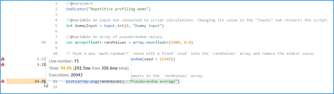
//@version=5
indicator("Repetitive profiling demo")

//@variable An input not connected to script calculations. Changing its value in the "Inputs" tab restarts the script.
int dummyInput = input.int(0, "Dummy input")

//@variable An array of pseudorandom values.
var array<float> randValues = array.new<float>(2500, 0.0)

// Push a new `math.random()` value with a fixed `seed` into the `randValues` array and remove the oldest value.
array.push(randValues, math.random(seed = 12345))
array.shift(randValues)

// Plot the average of all elements in the `randValues` array.
plot(array.avg(randValues), "Pseudorandom average")
第一次脚本运行后,Profiler 显示执行所有图表数据花费了 308.6 毫秒:
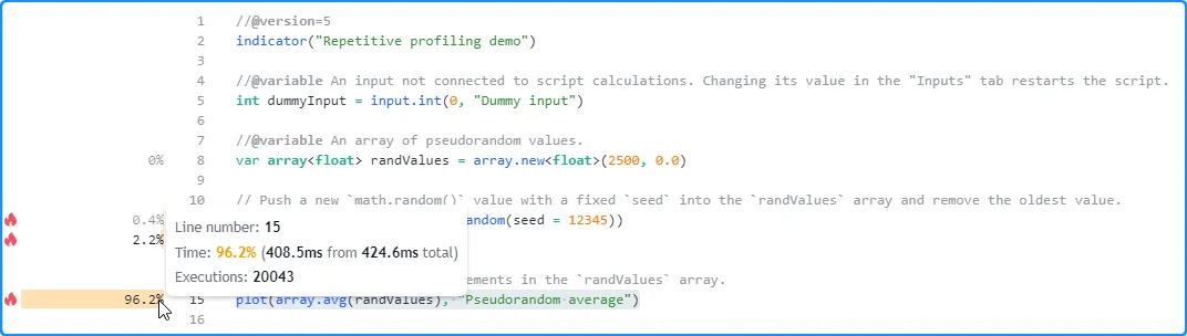
现在,让我们在脚本设置中更改虚拟输入的值,以重新启动它而不更改计算。这一次,它在 424.6 毫秒内完成了相同的代码执行,比上次运行长 116 毫秒:
再次重新启动脚本,结果又发生了变化。第三次运行时,脚本在 227.4 毫秒内完成了所有代码执行,这是迄今为止最短的时间:
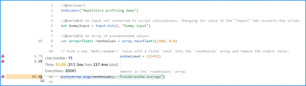
重复此过程几次并记录每次运行的结果后,可以手动计算它们的平均值来估计脚本的预期总运行时间:
AverageTime = (time1 + time2 + ... + timeN) / N
优化
代码优化(不要与指标或策略优化混淆)涉及修改脚本的源代码以缩短执行时间、提高资源效率和可扩展性。当程序员需要增强运行时性能时,他们可以使用各种方法来优化脚本,具体取决于脚本的计算内容。
从根本上讲,优化 Pine 代码所用的大部分技术都涉及减少关键计算的次数,或 用简化公式或内置公式替换重要计算。这两种范式经常重叠。
以下部分解释了程序员可以应用来优化其 Pine Script™ 代码的几个简单的概念。
使用内置函数
Pine Script™ 具有多种内置函数和变量,可帮助简化脚本创建。Pine 的许多内置函数都具有内部优化功能,可帮助最大限度地提高效率并最大限度地缩短执行时间。因此,优化 Pine 代码的最简单方法之一是尽可能在脚本的计算中利用这些高效的内置函数。
让我们看一个例子,其中可以用简洁的内置调用替换用户定义的计算,以大幅提高性能。假设程序员想要计算指定数量的条形图的系列的最高值。不熟悉 Pine 所有内置功能的人可能会使用如下代码来完成任务,该代码
在每个条形图上使用循环length来比较系列的历史值source:
//@variable A user-defined function to calculate the highest `source` value over `length` bars.
pineHighest(float source, int length) =>
    float result = na
    if bar_index + 1 >= length
        result := source
        if length > 1
            for i = 1 to length - 1
                result := math.max(result, source[i])
    result
或者,可以通过减少循环执行的次数来设计更优化的 Pine 函数,因为source仅在特定条件发生时才需要迭代历史记录以获得结果:
//@variable A faster user-defined function to calculate the highest `source` value over `length` bars.
//          This version only requires a loop when the highest value is removed from the window, the `length`
//          changes, or when the number of bars first becomes sufficient to calculate the result.
fasterPineHighest(float source, int length) =>
    var float result = na
    if source[length] == result or length != length[1] or bar_index + 1 == length
        result := source
        if length > 1
            for i = 1 to length - 1
                result := math.max(result, source[i])
    else
        result := math.max(result, source)
    result
内置的
ta.highest()
函数将优于这两种pineHighest()实现,因为其内部计算经过高度优化,可实现高效执行。下面,我们创建了一个脚本,绘制了调用、fasterPineHighest()和
ta.highest()的结果,
以使用Profiler
比较它们的性能
:
//@version=5
indicator("Using built-ins demo")

//@variable A user-defined function to calculate the highest `source` value over `length` bars.
pineHighest(float source, int length) =>
    float result = na
    if bar_index + 1 >= length
        result := source
        if length > 1
            for i = 1 to length - 1
                result := math.max(result, source[i])
    result

//@variable A faster user-defined function to calculate the highest `source` value over `length` bars.
//          This version only requires a loop when the highest value is removed from the window, the `length`
//          changes, or when the number of bars first becomes sufficient to calculate the result.
fasterPineHighest(float source, int length) =>
    var float result = na
    if source[length] == result or length != length[1] or bar_index + 1 == length
        result := source
        if length > 1
            for i = 1 to length - 1
                result := math.max(result, source[i])
    else
        result := math.max(result, source)
    result

plot(pineHighest(close, 20))
plot(fasterPineHighest(close, 20))
plot(ta.highest(close, 20))
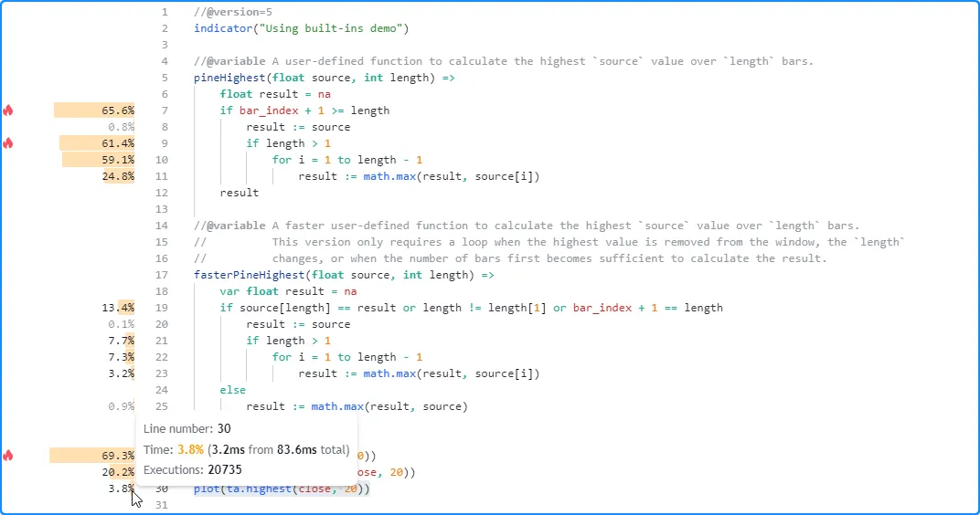
对 20,735 次脚本执行的
分析结果显示
,对 的调用pineHighest()执行时间最长,运行时间为 57.9 毫秒,约占脚本总运行时间的 69.3%。该
fasterPineHighest()调用的执行效率更高,因为它仅花费约 16.9 毫秒(约占总运行时间的 20.2%)来计算相同的值。
然而, 迄今为止最有效的是ta.highest() 调用,它只需要 3.2 毫秒(约占总运行时间的 3.8%)即可执行所有图表的数据并在本次运行中计算相同的值:
虽然这些结果有效地证明了内置函数的性能优于
带有 20 个小参数的用户定义函数length,但必须考虑到函数所需的计算将
随参数的值而变化。因此,我们可以在使用
不同参数时对代码进行性能分析,以衡量其运行时的扩展情况。
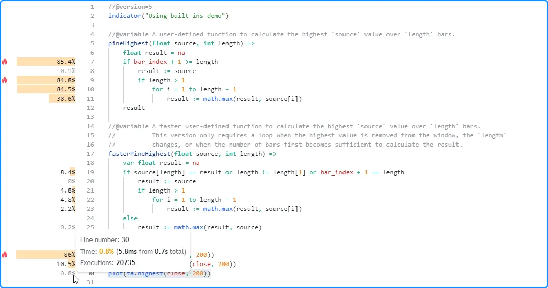
在这里,我们将length每个函数调用中的参数从 20 更改为 200,然后
再次分析脚本以观察性能变化。pineHighest()本次运行中该函数所花费的时间增加到约 0.6 秒(约占总运行时间的 86%),该
fasterPineHighest()函数所花费的时间增加到约 75 毫秒。
另一方面,ta.highest()函数的运行时间没有发生显著变化。这次大约花费了 5.8 毫秒,仅比上次运行多了几毫秒。
换句话说,虽然我们的
用户定义函数在本次运行中由于参数增加而经历了显著的运行时间增长
length,但内置
ta.highest()
函数的运行时间变化在这种情况下相对较小,从而进一步强调了其性能优势:
注意:
- 在许多情况下,脚本的运行时可受益于使用内置函数(如果适用)。但是,使用内置函数所实现的相对性能优势取决于脚本的 高影响代码和所使用的特定内置函数。无论如何,在探索优化解决方案时,应始终 对其脚本进行性能分析(最好是 多次)。
- 本例中函数执行的计算也取决于图表数据的顺序。因此,程序员也可以通过跨 不同数据集分析脚本来进一步了解其总体性能。
减少重复
Pine Script™ 编译器可以自动简化某些类型的 重复代码,无需程序员干预。但是,这种自动过程有其局限性。如果脚本包含编译器无法减少的重复计算,程序员可以手动减少重复以提高脚本的性能。
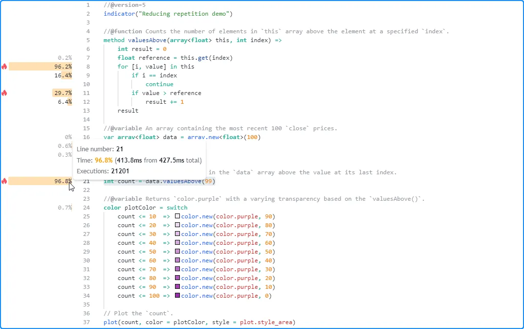
例如,此脚本包含一个valuesAbove()
方法
,该方法计算数组中指定索引处元素上方的元素数量
。该脚本使用计算的绘制数组
最后一个索引处元素上方的值数量。它计算在switch
结构中
调用其所有 10 个条件表达式的:dataplotColorplotColorvaluesAbove()
//@version=5
indicator("Reducing repetition demo")

//@function Counts the number of elements in `this` array above the element at a specified `index`.
method valuesAbove(array<float> this, int index) =>
    int result = 0
    float reference = this.get(index)
    for [i, value] in this
        if i == index
            continue
        if value > reference
            result += 1
    result

//@variable An array containing the most recent 100 `close` prices.
var array<float> data = array.new<float>(100)
data.push(close)
data.shift()

//@variable Returns `color.purple` with a varying transparency based on the `valuesAbove()`.
color plotColor = switch
    data.valuesAbove(99) <= 10  => color.new(color.purple, 90)
    data.valuesAbove(99) <= 20  => color.new(color.purple, 80)
    data.valuesAbove(99) <= 30  => color.new(color.purple, 70)
    data.valuesAbove(99) <= 40  => color.new(color.purple, 60)
    data.valuesAbove(99) <= 50  => color.new(color.purple, 50)
    data.valuesAbove(99) <= 60  => color.new(color.purple, 40)
    data.valuesAbove(99) <= 70  => color.new(color.purple, 30)
    data.valuesAbove(99) <= 80  => color.new(color.purple, 20)
    data.valuesAbove(99) <= 90  => color.new(color.purple, 10)
    data.valuesAbove(99) <= 100 => color.new(color.purple, 0)

// Plot the number values in the `data` array above the value at its last index.
plot(data.valuesAbove(99), color = plotColor, style = plot.style_area)
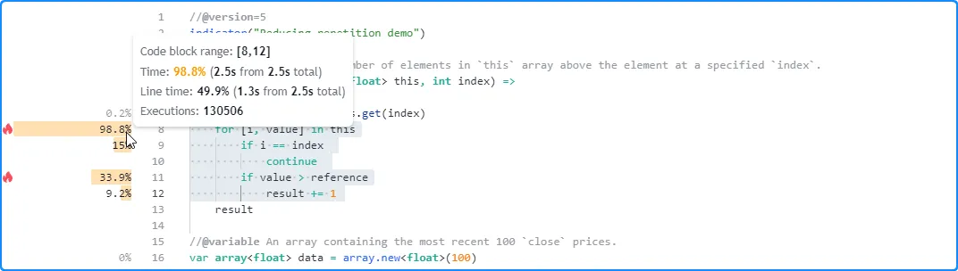
此脚本的分析结果显示
,它执行了 21,201 次,耗时约 2.5 秒。对脚本运行时影响最大的代码区域是
从第 8 行开始的本地范围
内的for循环和从第 21 行开始的switch
块:valuesAbove()
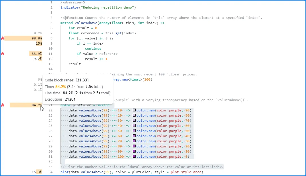
请注意,显示的本地代码的执行次数
valuesAbove()远远大于脚本全局范围内的代码的执行次数,因为脚本每次执行最多调用该方法 11 次,而函数
本地代码的结果反映了每次单独调用的总时间和执行次数:
尽管每次valuesAbove()调用都使用相同的参数并返回相同的结果,但编译器无法在翻译过程中自动为我们减少此代码。我们需要自己完成这项工作。我们可以通过将的值分配data.valuesAbove(99)给变量并在需要结果的所有其他区域中重复使用该值来优化此脚本。
在下面的版本中,我们通过添加一个count
变量来引用该data.valuesAbove(99)值来修改脚本。脚本在plotColor计算和
plot()
调用中使用此变量:
//@version=5
indicator("Reducing repetition demo")

//@function Counts the number of elements in `this` array above the element at a specified `index`.
method valuesAbove(array<float> this, int index) =>
    int result = 0
    float reference = this.get(index)
    for [i, value] in this
        if i == index
            continue
        if value > reference
            result += 1
    result

//@variable An array containing the most recent 100 `close` prices.
var array<float> data = array.new<float>(100)
data.push(close)
data.shift()

//@variable The number values in the `data` array above the value at its last index.
int count = data.valuesAbove(99)

//@variable Returns `color.purple` with a varying transparency based on the `valuesAbove()`.
color plotColor = switch
    count <= 10  => color.new(color.purple, 90)
    count <= 20  => color.new(color.purple, 80)
    count <= 30  => color.new(color.purple, 70)
    count <= 40  => color.new(color.purple, 60)
    count <= 50  => color.new(color.purple, 50)
    count <= 60  => color.new(color.purple, 40)
    count <= 70  => color.new(color.purple, 30)
    count <= 80  => color.new(color.purple, 20)
    count <= 90  => color.new(color.purple, 10)
    count <= 100 => color.new(color.purple, 0)

// Plot the `count`.
plot(count, color = plotColor, style = plot.style_area)
经过此修改,
分析结果显示性能显著提高,因为脚本现在只需要在每次执行时评估一次valuesAbove()调用,而不是最多 11 次:
注意:
尽量减少 `request.*()`调用
命名空间中的内置函数允许脚本从其他上下文request.*()中检索数据
。虽然这些函数在许多应用程序中都提供了实用性,但重要的是要考虑到每次调用这些函数都会对脚本的资源使用产生重大影响。
单个脚本最多可以包含 40 次对request.*()函数系列的调用。但是,用户应努力将脚本的
request.*()调用次数保持在此限制以下,以尽可能降低数据请求对性能的影响。
当脚本使用多个
request.security()
或
request.security_lower_tf()调用从同一上下文请求多个表达式的值时
,优化此类请求的一种有效方法是将它们压缩为使用
元组作为参数的单个调用。这种优化不仅有助于缩短请求的运行时间,还有助于减少脚本的内存使用量和编译大小。request.*()expression
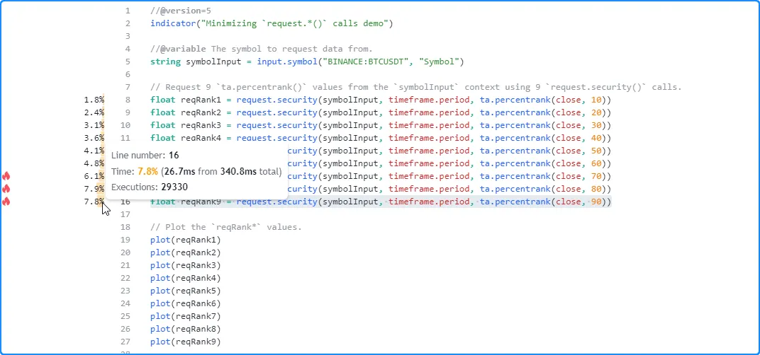
举一个简单的例子,以下脚本 使用对request.security() 的九个单独调用从指定符号请求具有不同长度的 九个ta.percentrank()值。然后,它将所有九个请求的值绘制在图表上,以在输出中使用它们:
//@version=5
indicator("Minimizing `request.*()` calls demo")

//@variable The symbol to request data from.
string symbolInput = input.symbol("BINANCE:BTCUSDT", "Symbol")

// Request 9 `ta.percentrank()` values from the `symbolInput` context using 9 `request.security()` calls.
float reqRank1 = request.security(symbolInput, timeframe.period, ta.percentrank(close, 10))
float reqRank2 = request.security(symbolInput, timeframe.period, ta.percentrank(close, 20))
float reqRank3 = request.security(symbolInput, timeframe.period, ta.percentrank(close, 30))
float reqRank4 = request.security(symbolInput, timeframe.period, ta.percentrank(close, 40))
float reqRank5 = request.security(symbolInput, timeframe.period, ta.percentrank(close, 50))
float reqRank6 = request.security(symbolInput, timeframe.period, ta.percentrank(close, 60))
float reqRank7 = request.security(symbolInput, timeframe.period, ta.percentrank(close, 70))
float reqRank8 = request.security(symbolInput, timeframe.period, ta.percentrank(close, 80))
float reqRank9 = request.security(symbolInput, timeframe.period, ta.percentrank(close, 90))

// Plot the `reqRank*` values.
plot(reqRank1)
plot(reqRank2)
plot(reqRank3)
plot(reqRank4)
plot(reqRank5)
plot(reqRank6)
plot(reqRank7)
plot(reqRank8)
plot(reqRank9)
对脚本进行分析的结果 显示,脚本花费了 340.8 毫秒来完成其请求并绘制此运行中的值:
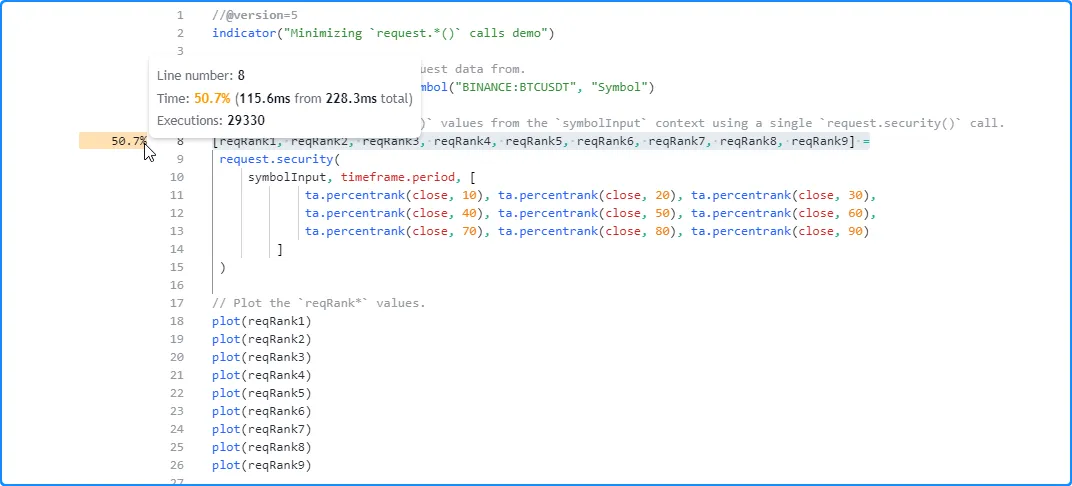
由于所有
request.security()调用都从同一上下文
请求数据,我们可以将它们全部合并到使用
元组作为参数的单个request.security()
调用中,
从而优化代码的资源使用情况:expression
//@version=5
indicator("Minimizing `request.*()` calls demo")

//@variable The symbol to request data from.
string symbolInput = input.symbol("BINANCE:BTCUSDT", "Symbol")

// Request 9 `ta.percentrank()` values from the `symbolInput` context using a single `request.security()` call.
[reqRank1, reqRank2, reqRank3, reqRank4, reqRank5, reqRank6, reqRank7, reqRank8, reqRank9] =
 request.security(
     symbolInput, timeframe.period, [
             ta.percentrank(close, 10), ta.percentrank(close, 20), ta.percentrank(close, 30),
             ta.percentrank(close, 40), ta.percentrank(close, 50), ta.percentrank(close, 60),
             ta.percentrank(close, 70), ta.percentrank(close, 80), ta.percentrank(close, 90)
         ]
 )

// Plot the `reqRank*` values.
plot(reqRank1)
plot(reqRank2)
plot(reqRank3)
plot(reqRank4)
plot(reqRank5)
plot(reqRank6)
plot(reqRank7)
plot(reqRank8)
plot(reqRank9)
正如我们在下面看到的, 运行此版本脚本的分析结果显示,这次花费了 228.3 毫秒,比上次运行有了很大的改进:
注意:
- 脚本可用的计算资源会随时间波动 。因此, 多次分析脚本有助于巩固性能结论,这通常是一个好主意。
- 另一种通过一次调用从同一上下文请求多个值的方法
request.*()是将 用户定义类型 (UDT)的 对象作为参数传递。请参阅 其他时间范围和数据页面的 此部分,了解有关请求 UDT 的更多信息。expression - 程序员还可以
通过向函数的参数传递实参来减少request.security()、
request.security_lower_tf()或
request.seed()
calc_bars_count调用的总运行时间 ,这会限制它可以从上下文访问并执行所需计算的历史数据点的数量。通常,如果对这些request.*()函数的调用检索的历史数据多于脚本 所需的数据,则限制请求calc_bars_count可以帮助提高脚本的性能。
避免重绘
Pine Script™ 的 绘图类型允许脚本在图表上绘制自定义视觉效果,而这是通过其他输出(例如 绘图)无法实现的。虽然这些类型提供了更大的视觉灵活性,但它们的运行时间和内存成本也更高,尤其是当脚本不必要地重新创建 绘图而不是直接更新其属性以更改其外观时。
大多数 绘图类型(折线除外 )的命名空间中都具有内置的设置器函数,允许脚本修改绘图而无需删除并重新创建绘图。当仅特定属性需要修改时,使用这些设置器通常比创建新绘图对象所需的计算成本更低。
例如,下面的脚本将删除和重新绘制
框与使用
box.set*()函数进行比较。在第一个栏上,它声明redrawnBoxes
和updatedBoxes 数组
并执行循环以将 25 个框
元素推送到其中。
该脚本使用单独的
for循环遍历数组并在每次执行时更新绘图。它使用
box.delete()
和
box.new()重新创建数组中的
框,而使用
box.set_lefttop()
和
box.set_rightbottom()直接修改数组中
框的属性
。两种方法都实现了相同的视觉效果。但是,后者效率更高:redrawnBoxesupdatedBoxes
//@version=5
indicator("Avoiding redrawing demo")

//@variable An array of `box` IDs deleted with `box.delete()` and redrawn with `box.new()` on each execution.
var array<box> redrawnBoxes = array.new<box>()
//@variable An array of `box` IDs with properties that update across executions update via `box.set*()` functions.
var array<box> updatedBoxes = array.new<box>()

// Populate both arrays with 25 elements on the first bar.
if barstate.isfirst
    for i = 1 to 25
        array.push(redrawnBoxes, box(na))
        array.push(updatedBoxes, box.new(na, na, na, na))

for i = 0 to 24
    // Calculate coordinates.
    int x = bar_index - i
    float y = close[i + 1] - close
    // Get the `box` ID from each array at the `i` index.
    box redrawnBox = redrawnBoxes.get(i)
    box updatedBox = updatedBoxes.get(i)
    // Delete the `redrawnBox`, create a new `box` ID, and replace that element in the `redrawnboxes` array.
    box.delete(redrawnBox)
    redrawnBox := box.new(x - 1, y, x, 0.0)
    array.set(redrawnBoxes, i, redrawnBox)
    // Update the properties of the `updatedBox` rather than redrawing it.
    box.set_lefttop(updatedBox, x - 1, y)
    box.set_rightbottom(updatedBox, x, 0.0)
对该脚本进行性能分析的结果 显示,包含 box.new() 调用的第 24 行是每个条形图上执行的 代码块中 最繁重的行,其运行时间接近第 27 行和第 28 行上box.set_lefttop() 和 box.set_rightbottom()调用所花费时间总和 的两倍 :
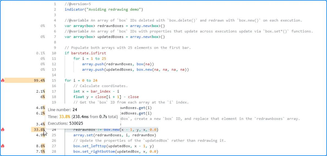
注意:
- 循环本地代码显示的执行次数是脚本全局范围内代码显示次数的 25 倍,因为每次执行循环语句都会触发 25 次本地块的执行。
- 此脚本会更新图表历史记录中所有条形图的绘图,以用于测试目的。但是,它实际上并不 需要执行所有这些历史更新,因为用户只会看到最后一个历史条形图的最终结果和实时条形图的变化。请参阅 下一节以了解更多信息。
减少图纸更新
当脚本生成 随历史条形图变化的绘图对象时,用户只能在这些条形图上看到最终结果,因为脚本在首次加载到图表上时就完成了其历史执行。只有在实时条形图期间,随着新数据的流入,才能看到此类绘图随执行 而变化。
由于用户永远看不到历史条形图上动态绘图的不断变化的输出 ,因此通常可以通过消除不影响最终结果的历史更新来提高脚本的性能。
例如,此脚本创建一个
包含两列和 21 行的
表格,以
分页表格格式
可视化RSIinfoTable的历史记录。该脚本初始化第一条柱上的单元格,并引用计算的历史记录rsi来更新
text每条柱上的forbgcolor循环内第二列单元格的单元
格:
//@version=5
indicator("Reducing drawing updates demo")

//@variable The first offset shown in the paginated table.
int offsetInput = input.int(0, "Page", 0, 249) * 20

//@variable A table that shows the history of RSI values.
var table infoTable = table.new(position.top_right, 2, 21, border_color = chart.fg_color, border_width = 1)
// Initialize the table's cells on the first bar.
if barstate.isfirst
    table.cell(infoTable, 0, 0, "Offset", text_color = chart.fg_color)
    table.cell(infoTable, 1, 0, "RSI", text_color = chart.fg_color)
    for i = 0 to 19
        table.cell(infoTable, 0, i + 1, str.tostring(offsetInput + i))
        table.cell(infoTable, 1, i + 1)

float rsi = ta.rsi(close, 14)

// Update the history shown in the `infoTable` on each bar.
for i = 0 to 19
    float historicalRSI = rsi[offsetInput + i]
    table.cell_set_text(infoTable, 1, i + 1, str.tostring(historicalRSI))
    table.cell_set_bgcolor(
         infoTable, 1, i + 1, color.from_gradient(historicalRSI, 30, 70, color.red, color.green)
     )

plot(rsi, "RSI")
对脚本进行性能分析后 ,我们发现对性能影响最大的代码是 从第 20 行开始的for循环,即 更新表格单元格的代码块:
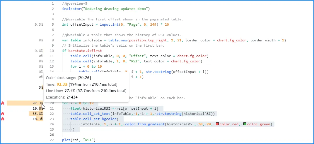
此关键代码区域在图表的历史记录中 执行过多,因为用户只能看到表格的 最终 历史结果。用户唯一能看到 表格 更新的时间是在最后一个历史条形图上以及所有后续 实时条形图上。因此,我们可以将此代码的执行限制在最后一个可用条形图上,从而优化此脚本的资源使用情况。
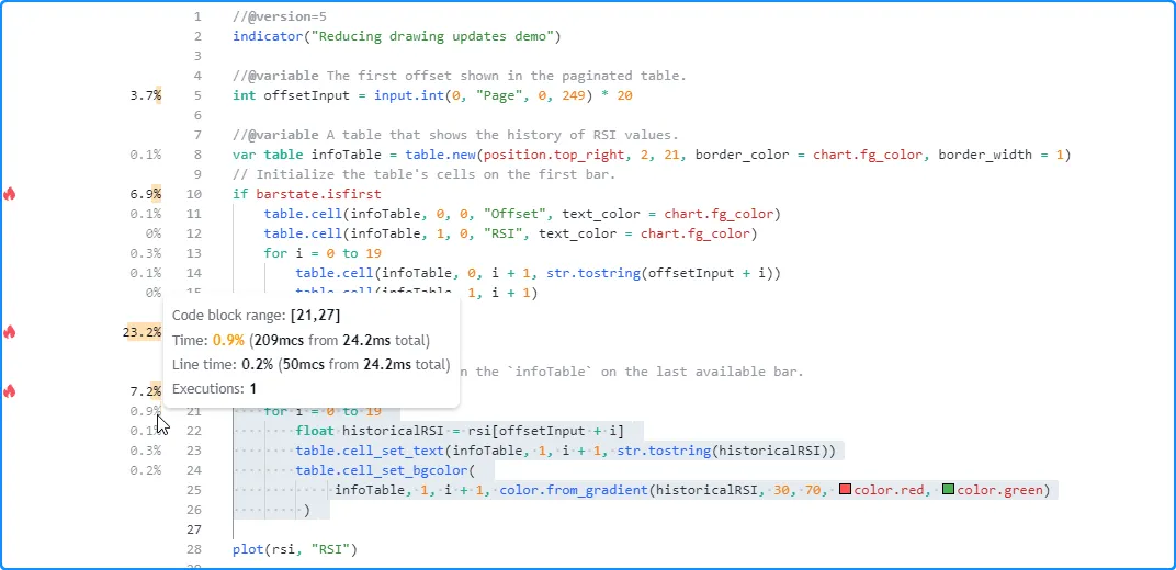
在此脚本版本中,我们将 更新 表格单元格的循环放在 使用 barstate.islast 作为条件的 if结构 中 ,从而有效地将代码块的执行限制为仅最后一个历史条和所有实时条。现在,脚本加载效率更高,因为所有表格的计算只需要一次历史执行:
//@version=5
indicator("Reducing drawing updates demo")

//@variable The first offset shown in the paginated table.
int offsetInput = input.int(0, "Page", 0, 249) * 20

//@variable A table that shows the history of RSI values.
var table infoTable = table.new(position.top_right, 2, 21, border_color = chart.fg_color, border_width = 1)
// Initialize the table's cells on the first bar.
if barstate.isfirst
    table.cell(infoTable, 0, 0, "Offset", text_color = chart.fg_color)
    table.cell(infoTable, 1, 0, "RSI", text_color = chart.fg_color)
    for i = 0 to 19
        table.cell(infoTable, 0, i + 1, str.tostring(offsetInput + i))
        table.cell(infoTable, 1, i + 1)

float rsi = ta.rsi(close, 14)

// Update the history shown in the `infoTable` on the last available bar.
if barstate.islast
    for i = 0 to 19
        float historicalRSI = rsi[offsetInput + i]
        table.cell_set_text(infoTable, 1, i + 1, str.tostring(historicalRSI))
        table.cell_set_bgcolor(
             infoTable, 1, i + 1, color.from_gradient(historicalRSI, 30, 70, color.red, color.green)
         )

plot(rsi, "RSI")
注意:
- 当新的实时 更新出现时,脚本仍会更新单元格,因为用户可以在图表上观察到这些变化,这与脚本在历史条上执行的变化不同。
存储计算值
当脚本执行关键计算且 在整个执行过程中很少发生变化时,可以通过 将结果保存到使用var或 varip关键字声明的变量中 并仅在计算发生变化时更新该值来减少其运行时间。如果脚本计算多个值过多,则可以将它们存储在 集合、 矩阵、 映射或 用户定义类型的 对象中。
让我们看一个例子。此脚本根据广义窗口函数计算具有自定义权重的加权移动平均值。
是加权收盘numerator价的总和
,是计算出的权重的总和。该脚本使用
for循环迭代多次来计算这些总和,然后绘制它们的比率,即最终的平均值:denominatorlengthInput
//@version=5
indicator("Storing calculated values demo", overlay = true)

//@variable The number of bars in the weighted average calculation.
int lengthInput = input.int(50, "Length", 1, 5000)
//@variable Window coefficient.
float coefInput = input.float(0.5, "Window coefficient", 0.0, 1.0, 0.01)

//@variable The sum of weighted `close` prices.
float numerator = 0.0
//@variable The sum of weights.
float denominator = 0.0

//@variable The angular step in the cosine calculation.
float step = 2.0 * math.pi / lengthInput
// Accumulate weighted sums.
for i = 0 to lengthInput - 1
    float weight = coefInput - (1 - coefInput) * math.cos(step * i)
    numerator += close[i] * weight
    denominator += weight

// Plot the weighted average result.
plot(numerator / denominator, "Weighted average", color.purple, 3)
在 根据我们的图表数据对脚本的性能进行分析之后,我们发现,计算 20,155 个图表更新的默认 50 条平均值大约需要 241.3 毫秒,而 对脚本性能 影响最大的关键代码是从第 17 行开始的循环块:
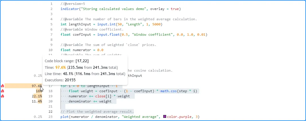
由于循环迭代次数取决于该lengthInput
值,让我们测试一下它的运行时间如何与
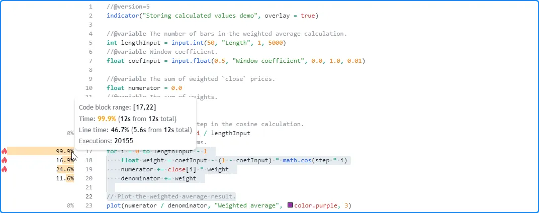
需要更重循环的另一个配置一起扩展。在这里,我们将值设置为 2500。这次,脚本大约需要 12 秒才能完成所有执行:
现在我们已经确定了脚本中影响最大的代码,并建立了改进基准,我们可以检查关键代码块以识别优化机会。检查计算后,我们可以观察到以下内容:
weight导致第 18 行的计算在循环迭代中发生变化的唯一值是循环索引。其计算中的所有其他值保持一致。因此,weight每次循环迭代计算的在图表条形图中不会发生变化。因此,我们不必在每次更新时都计算权重,而是可以在第一个条形图上计算一次,然后 将它们存储在集合中 ,以便在后续脚本执行中访问。- 由于权重永远不会改变,结果也
denominator永远不会改变。因此,我们可以 在 变量声明中添加var关键字,并只计算一次其值,以减少执行加法赋值运算的次数 。 - 与 不同
denominator,我们无法存储该numerator值以简化其计算,因为它会随着时间的推移不断变化。
在下面修改后的脚本中,我们添加了一个weights变量来引用
存储每个计算的 的数组weight。此变量和 都
在其声明中denominator包含
var
关键字,这意味着分配给它们的值将
在整个脚本执行过程中保持不变,直到明确重新分配。该脚本使用
仅在第一个图表条上执行的for循环来计算它们的值。在所有其他条中,它使用
引用数组中保存的值的for…in
循环来计算:numeratorweights
//@version=5
indicator("Storing calculated values demo", overlay = true)
//@variable The number of bars in the weighted average calculation.
int lengthInput = input.int(50, "Length", 1, 5000)
//@variable Window coefficient.
float coefInput = input.float(0.5, "Window coefficient", 0.0, 1.0, 0.01)
//@variable An array that stores the `weight` values calculated on the first chart bar.
var array<float> weights = array.new<float>()
//@variable The sum of weighted `close` prices.
float numerator = 0.0
//@variable The sum of weights. The script now only calculates this value on the first bar.
var float denominator = 0.0
//@variable The angular step in the cosine calculation.
float step = 2.0 * math.pi / lengthInput
// Populate the `weights` array and calculate the `denominator` only on the first bar.
if barstate.isfirst
for i = 0 to lengthInput - 1
float weight = coefInput - (1 - coefInput) * math.cos(step * i)
array.push(weights, weight)
denominator += weight
// Calculate the `numerator` on each bar using the stored `weights`.
for [i, w] in weights
numerator += close[i] * w
// Plot the weighted average result.
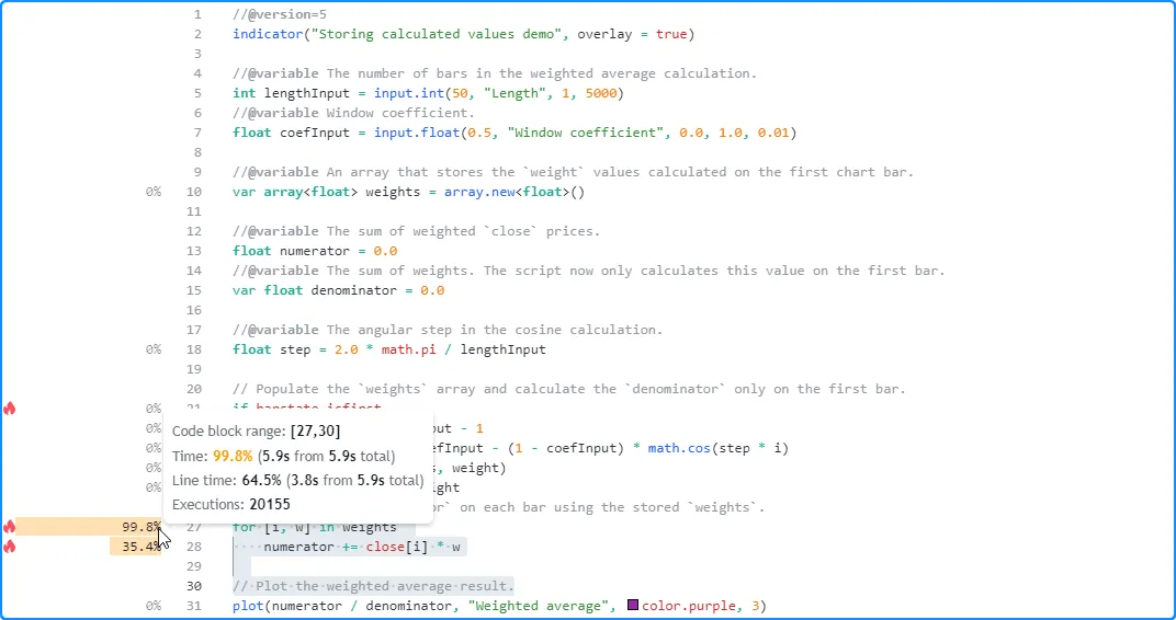
plot(numerator / denominator, "Weighted average", color.purple, 3)
通过这种优化的结构,
分析结果显示,我们修改后的脚本在高lengthInput
值为 2500 的情况下,对相同数据的计算大约需要 5.9 秒,大约是之前版本时间的一半:
注意:
- 尽管我们通过将其执行不变的值保存到变量中显著提高了此脚本的性能,但由于在每个条上执行的剩余循环计算,它在大 值的情况下仍然涉及更高的计算成本。
lengthInput - 另一种更高级的方法是,将权重存储在
第一条柱上的
单行
矩阵中,使用数组
作为
队列来保存最近的
收盘
价,然后用
对matrix.mult()
的调用
替换for…in循环。请参阅矩阵
页面以了解有关使用函数的更多信息。
matrix.*()
消除环路
循环允许 Pine 脚本在每次执行时进行迭代计算。每次激活循环时,其本地代码可能会执行多次,这通常会导致资源使用量大幅增加。
Pine 循环对于某些计算是必需的,例如操作 集合中的元素或回顾数据集的历史记录以计算仅在当前栏上可获得的值。然而,在许多其他情况下,程序员在不需要时使用循环,导致运行时性能不佳。在这种情况下,可以根据计算内容通过以下任何一种方式消除不必要的循环:
- 识别无需迭代即可实现相同结果的简化、无循环表达式
- 尽可能使用优化的内置函数替换循环
- 在可行的情况下将循环迭代分散到各个条形中,而不是一次性评估所有条形
这个简单的例子包含一个avgDifference()函数,用于计算当前柱线source
值与之前柱线所有值之间的平均差值length。脚本调用此函数来计算当前
收盘
价与lengthInput之前价格之间的平均差值,然后将
结果绘制在图表上:
//@version=5
indicator("Eliminating loops demo")
//@variable The number of bars in the calculation.
int lengthInput = input.int(20, "Length", 1)
//@function Calculates the average difference between the current `source` and `length` previous `source` values.
avgDifference(float source, int length) =>
float diffSum = 0.0
for i = 1 to length
diffSum += source - source[i]
diffSum / length
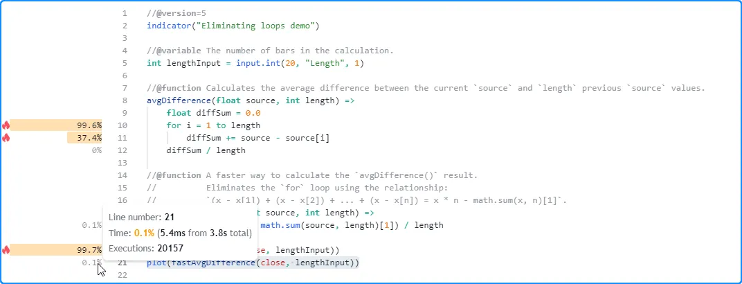
plot(avgDifference(close, lengthInput))
在使用默认设置检查脚本的 分析结果后,我们发现执行 20,157 次大约需要 64 毫秒:
由于我们在调用中
使用了lengthInput作为参数,并且该参数控制函数内部循环必须迭代的次数,因此我们的脚本的运行时间将
随着值的增长而增长。在这里,我们在脚本的设置中将输入的值设置为 2000。这次,脚本在大约 3.8 秒内完成了执行:lengthavgDifference()lengthInput
从这些结果中我们可以看出,由于函数
在每个柱上执行
foravgDifference()循环,因此调用该函数的成本可能很高,具体取决于指定的值。但是,循环对于实现输出来说并不是必需的。为了理解原因,让我们仔细看看循环的计算。我们可以用以下表达式表示它们:lengthInput
(source - source[1]) + (source - source[2]) + ... + (source - source[length])
请注意,它将当前 source值乘以length。这些迭代加法不是必需的。我们可以将表达式的该部分简化为source * length,从而将其简化为以下内容:
source * length - source[1] - source[2] - ... - source[length]
或者等价地:
source * length - (source[1] + source[2] + ... + source[length])
简化并重新排列循环计算的表示后,我们发现,我们可以用更简单的方式计算结果,并
通过从值中减去前一个条形的滚动值总和
来消除循环,即:sourcesource * length
source * length - math.sum(source, length)[1]
下面的函数fastAvgDifference()是原始函数的无循环avgDifference()替代,它使用上面的表达式来计算差异的总和source,然后将表达式除以length返回平均差异:
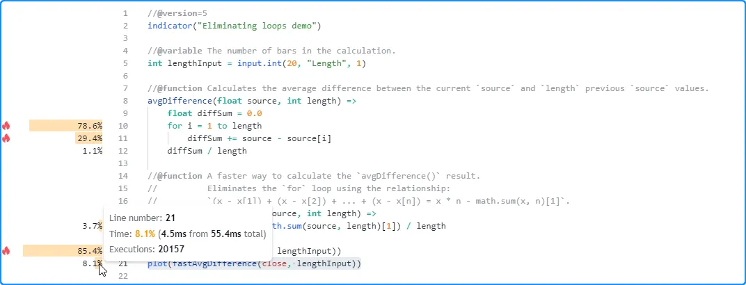
//@function A faster way to calculate the `avgDifference()` result.
//          Eliminates the `for` loop using the relationship:
//          `(x - x[1]) + (x - x[2]) + ... + (x - x[n]) = x * n - math.sum(x, n)[1]`.
fastAvgDifference(float source, int length) =>
    (source * length - math.sum(source, length)[1]) / length
现在我们已经确定了一个潜在的优化解决方案,我们可以将 的性能fastAvgDifference()与原始
avgDifference()函数进行比较。下面的脚本是以前版本的修改形式,它绘制了使用 作为参数调用两个函数的lengthInput结果length:
//@version=5
indicator("Eliminating loops demo")

//@variable The number of bars in the calculation.
int lengthInput = input.int(20, "Length", 1)

//@function Calculates the average difference between the current `source` and `length` previous `source` values.
avgDifference(float source, int length) =>
    float diffSum = 0.0
    for i = 1 to length
        diffSum += source - source[i]
    diffSum / length

//@function A faster way to calculate the `avgDifference()` result.
//          Eliminates the `for` loop using the relationship:
//          `(x - x[1]) + (x - x[2]) + ... + (x - x[n]) = x * n - math.sum(x, n)[1]`.
fastAvgDifference(float source, int length) =>
    (source * length - math.sum(source, length)[1]) / length

plot(avgDifference(close, lengthInput))
plot(fastAvgDifference(close, lengthInput))
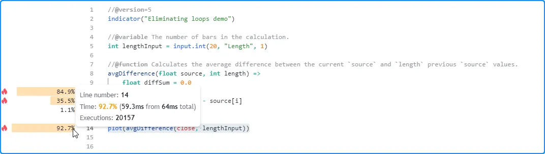
脚本的默认设置是 20,分析
结果lengthInput显示两次函数调用的运行时间存在显著差异。原始函数的调用在这次运行中执行了 20,157 次,耗时约 47.3 毫秒,而我们优化后的函数仅耗时 4.5 毫秒:
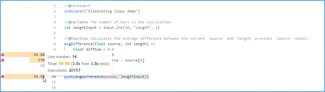
现在,让我们将性能与2000 这个更大的 lengthInput
值进行比较。与以前一样,avgDifference()
函数所花费的运行时间显著增加。但是,执行调用所花费的时间
fastAvgDifference()仍然非常接近以前
配置的结果。换句话说,虽然我们原始函数的运行时间与其length参数直接相关,但我们优化的函数表现出相对一致的性能,因为它不需要循环:
优化循环
尽管 Pine 的 执行模型和可用的内置函数通常在许多情况下消除了对循环的需要 ,但在某些情况下脚本仍需要循环来 执行某些类型的任务,包括:
- 当可用的内置函数不够用时,操作 集合或对集合的元素执行计算
- 执行跨历史条形图的计算,这是 使用简化的无循环表达式或优化的 内置函数无法实现的
- 计算只能通过迭代获得的值
当脚本使用 程序员无法 消除的循环时,可以使用多种技术来减少其对性能的影响。本节介绍两种最常见、最有用的技术,它们可以帮助提高所需循环的效率。
减少循环计算
在循环的局部范围内执行的代码可能会对其整体运行时间产生倍增影响,因为每次执行循环语句时,它通常会触发局部代码的多次迭代。因此,程序员应努力通过消除不必要的结构、函数调用和操作来使循环的计算尽可能简单,以最大限度地降低性能影响,尤其是当脚本必须在所有执行过程中多次评估其循环时。
例如,此脚本包含一个函数,该函数根据指定数组filteredMA()中的元素计算最多length唯一值的移动平均值。该函数将唯一值排队到数组中,使用
for…in
循环迭代并计算和总和
,然后返回这些总和的比率。在循环中,只有当元素不是
na且元素为时,它才会将值添加到总和中。该脚本利用此
用户定义函数计算
按 a 过滤的最多 100 个唯一收盘价的平均值
,并在图表上绘制结果:sourcetruemask
sourcedata
datanumeratordenominatordatamaskindextruerandMask
//@version=5
indicator("Reducing loop calculations demo", overlay = true)

//@function Calculates a moving average of up to `length` unique `source` values filtered by a `mask` array.
filteredMA(float source, int length, array<bool> mask) =>
    // Raise a runtime error if the size of the `mask` doesn't equal the `length`.
    if mask.size() != length
        runtime.error("The size of the `mask` array used in the `filteredMA()` call must match the `length`.")
    //@variable An array containing `length` unique `source` values.
    var array<float> data = array.new<float>(length)
    // Queue unique `source` values into the `data` array.
    if not data.includes(source)
        data.push(source)
        data.shift()
    // The numerator and denominator of the average.
    float numerator   = 0.0
    float denominator = 0.0
    // Loop to calculate sums.
    for item in data
        if na(item)
            continue
        int index = array.indexof(data, item)
        if mask.get(index)
            numerator   += item
            denominator += 1.0
    // Return the average, or the last non-`na` average value if the current value is `na`.
    fixnan(numerator / denominator)

//@variable An array of 100 pseudorandom "bool" values.
var array<bool> randMask = array.new<bool>(100, true)
// Push the first element from `randMask` to the end and queue a new pseudorandom value.
randMask.push(randMask.shift())
randMask.push(math.random(seed = 12345) < 0.5)
randMask.shift()

// Plot the `filteredMA()` of up to 100 unique `close` values filtered by the `randMask`.
plot(filteredMA(close, 100, randMask))
在
对脚本进行性能分析后,我们发现执行 21,778 次大约需要两秒钟。对性能影响最大的代码是第 37 行的表达式,该表达式调用了该filteredMA()函数。在filteredMA()
函数范围内,
for…in
循环的影响最大,index循环范围内的计算(第 22 行)对循环运行时间的贡献最大:
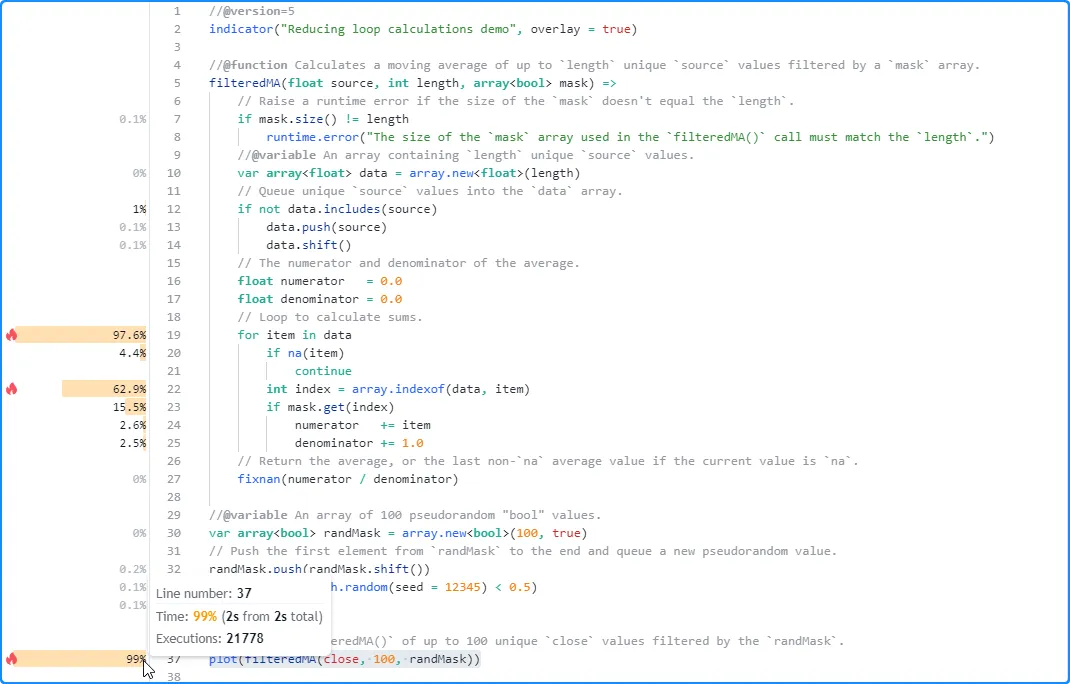
上述代码演示了
for…in
循环的次优用法,因为在这种情况下
我们不需要调用
array.indexof()
来检索。在循环中调用array.indexof()
函数的成本可能很高,因为每次脚本调用它时,它都必须搜索数组的
内容并找到相应元素的索引。index
为了消除 for...in 循环中这个代价高昂的调用,我们可以使用结构的 第二种形式,它在每次迭代中生成一个包含索引和元素值的元组:
for [index, item] in data
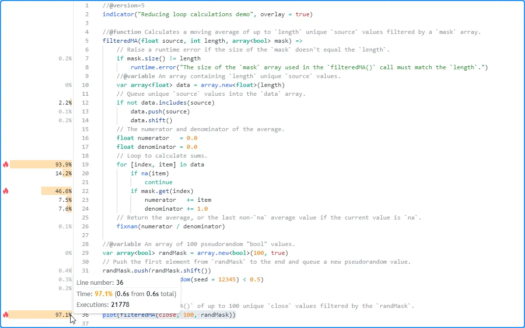
在此版本的脚本中,我们删除了 第 22 行的array.indexof() 调用,因为它对于实现预期结果 不是必需的,并且我们将for...in 循环更改为使用替代形式:
//@version=5
indicator("Reducing loop calculations demo", overlay = true)

//@function Calculates a moving average of up to `length` unique `source` values filtered by a `mask` array.
filteredMA(float source, int length, array<bool> mask) =>
    // Raise a runtime error if the size of the `mask` doesn't equal the `length`.
    if mask.size() != length
        runtime.error("The size of the `mask` array used in the `filteredMA()` call must match the `length`.")
    //@variable An array containing `length` unique `source` values.
    var array<float> data = array.new<float>(length)
    // Queue unique `source` values into the `data` array.
    if not data.includes(source)
        data.push(source)
        data.shift()
    // The numerator and denominator of the average.
    float numerator   = 0.0
    float denominator = 0.0
    // Loop to calculate sums.
    for [index, item] in data
        if na(item)
            continue
        if mask.get(index)
            numerator   += item
            denominator += 1.0
    // Return the average, or the last non-`na` average value if the current value is `na`.
    fixnan(numerator / denominator)

//@variable An array of 100 pseudorandom "bool" values.
var array<bool> randMask = array.new<bool>(100, true)
// Push the first element from `randMask` to the end and queue a new pseudorandom value.
randMask.push(randMask.shift())
randMask.push(math.random(seed = 12345) < 0.5)
randMask.shift()

// Plot the `filteredMA()` of up to 100 unique `close` values filtered by the `randMask`.
plot(filteredMA(close, 100, randMask))
通过这一简单的更改,我们的循环效率更高,因为它不再需要在每次迭代时重复搜索数组 来 跟踪索引。 此脚本运行的分析结果显示,它仅需 0.6 秒即可完成执行,与以前版本的结果相比有显著改进:
循环不变代码移动
循环不变代码是 循环范围内的任何代码区域,每次迭代都会产生不变的结果。当脚本的 循环包含循环不变代码时,由于过多、不必要的计算,在某些情况下可能会严重影响性能。
程序员可以通过将不变的计算移到循环范围之外来优化具有不变代码的循环,这样脚本只需在每次执行时评估一次它们,而不是重复评估。
以下示例包含一个函数,用于创建数组featureScale()的重新缩放版本
。在函数的
for…in
循环中,它通过计算每个元素与
array.min()的距离
并将值除以
array.range()来缩放每个元素。脚本使用此函数创建一个价格版本
,在图表上绘制rescaled.first()
和
rescaled.avg()值之间的差异
:rescaledarray and
//@version=5
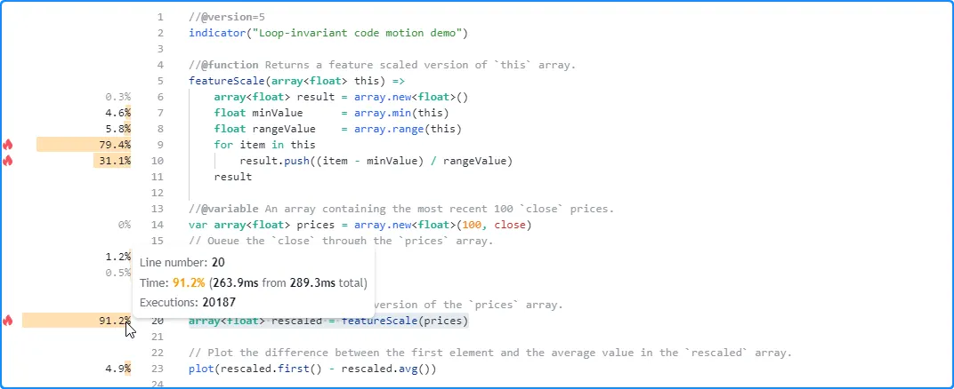
indicator("Loop-invariant code motion demo")
//@function Returns a feature scaled version of `this` array.
featureScale(array<float> this) =>
array<float> result = array.new<float>()
for item in this
result.push((item - array.min(this)) / array.range(this))
result
//@variable An array containing the most recent 100 `close` prices.
var array<float> prices = array.new<float>(100, close)
// Queue the `close` through the `prices` array.
prices.unshift(close)
prices.pop()
//@variable A feature scaled version of the `prices` array.
array<float> rescaled = featureScale(prices)
// Plot the difference between the first element and the average value in the `rescaled` array.
plot(rescaled.first() - rescaled.avg())
如下所示,
执行 20,187 次后,此脚本的分析结果显示它在大约 3.3 秒内完成运行。对性能影响最大的代码是包含函数featureScale()调用的行,而该函数的关键代码是
从第 7 行开始的 for…in
循环块:
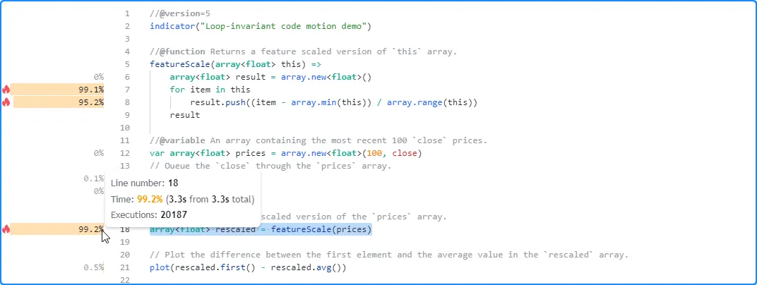
检查循环的计算后,我们可以看到 第 8 行的array.min() 和 array.range()调用是循环不变的,因为它们在每次迭代中始终会产生 相同的结果。我们可以将这些调用的结果分配给其范围之外的变量并根据需要引用它们,从而使循环更加高效 。
featureScale()以下脚本中的函数在执行 for…in 循环之前将 array.min() 和 array.range() 值分配
给和
变量。在
循环
的
局部minValue范围rangeValue内
,它在迭代过程中引用变量,而不是重复调用这些
函数:array.*()
//@version=5
indicator("Loop-invariant code motion demo")

//@function Returns a feature scaled version of `this` array.
featureScale(array<float> this) =>
    array<float> result = array.new<float>()
    float minValue      = array.min(this)
    float rangeValue    = array.range(this)
    for item in this
        result.push((item - minValue) / rangeValue)
    result

//@variable An array containing the most recent 100 `close` prices.
var array<float> prices = array.new<float>(100, close)
// Queue the `close` through the `prices` array.
prices.unshift(close)
prices.pop()

//@variable A feature scaled version of the `prices` array.
array<float> rescaled = featureScale(prices)

// Plot the difference between the first element and the average value in the `rescaled` array.
plot(rescaled.first() - rescaled.avg())
从脚本的 分析结果中我们可以看出,将循环不变计算移到循环之外可以显著提高性能。这次,脚本仅用 289.3 毫秒就完成了执行:
最小化历史缓冲区计算
Pine 脚本为其输出所依赖的所有变量和函数调用创建历史缓冲区。每个缓冲区都包含有关脚本可以使用历史引用运算符[]访问的历史值范围的信息 。
脚本通过分析数据集中前 244 个柱期间执行的历史引用,自动确定所有变量和函数调用所需的缓冲区大小。当脚本仅在这些初始柱之后引用计算值的历史记录时,它将在之前的柱中重复重新启动执行,并使用连续更大的历史缓冲区,直到确定合适的大小或引发运行时错误。在某些情况下,这些重复执行可能会显著增加脚本的运行时间。
当脚本在数据集中 过度执行以计算历史缓冲区时,提高其性能的一种有效方法是使用 max_bars_back()函数明确定义合适的缓冲区大小 。明确声明适当的缓冲区大小后,脚本无需在过去的数据中重新执行以确定大小。
例如,下面的脚本使用
折线
绘制一个基本直方图,表示
source500 个条形图上计算值的分布。在最后一个可用条形图上,脚本使用
for循环回顾计算source系列的历史值并确定
折线绘制使用的
图表点
。它还绘制了值以验证它执行的条形图数量:bar_index + 1
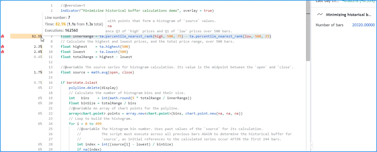
//@version=5
indicator("Minimizing historical buffer calculations demo", overlay = true)

//@variable A polyline with points that form a histogram of `source` values.
var polyline display = na
//@variable The difference Q3 of `high` prices and Q1 of `low` prices over 500 bars.
float innerRange = ta.percentile_nearest_rank(high, 500, 75) - ta.percentile_nearest_rank(low, 500, 25)
// Calculate the highest and lowest prices, and the total price range, over 500 bars.
float highest    = ta.highest(500)
float lowest     = ta.lowest(500)
float totalRange = highest - lowest

//@variable The source series for histogram calculation. Its value is the midpoint between the `open` and `close`.
float source = math.avg(open, close)

if barstate.islast
    polyline.delete(display)
    // Calculate the number of histogram bins and their size.
    int   bins    = int(math.round(5 * totalRange / innerRange))
    float binSize = totalRange / bins
    //@variable An array of chart points for the polyline.
    array<chart.point> points = array.new<chart.point>(bins, chart.point.new(na, na, na))
    // Loop to build the histogram.
    for i = 0 to 499
        //@variable The histogram bin number. Uses past values of the `source` for its calculation.
        //          The script must execute across all previous bars AGAIN to determine the historical buffer for
        //          `source`, as initial references to the calculated series occur AFTER the first 244 bars.
        int index = int((source[i] - lowest) / binSize)
        if na(index)
            continue
        chart.point currentPoint = points.get(index)
        if na(currentPoint.index)
            points.set(index, chart.point.from_index(bar_index + 1, (index + 0.5) * binSize + lowest))
            continue
        currentPoint.index += 1
    // Add final points to the `points` array and draw the new `display` polyline.
    points.unshift(chart.point.now(lowest))
    points.push(chart.point.now(highest))
    display := polyline.new(points, closed = true)

plot(bar_index + 1, "Number of bars", display = display.data_window)
由于脚本仅引用最后一条柱状图source的过去值,因此它不会在较大的数据集的前 244 条柱状图内为该系列构建合适的历史缓冲区。因此,它将在所有历史柱状图上重新执行以确定适当的缓冲区大小。
从脚本在 20,320 个柱状图上运行后的分析结果中可以看出
,全局代码执行次数
为 162,560 次,是图表柱状图数量的八倍。换句话说,脚本必须重复历史执行七次source才能确定本例中适合该系列的缓冲区:
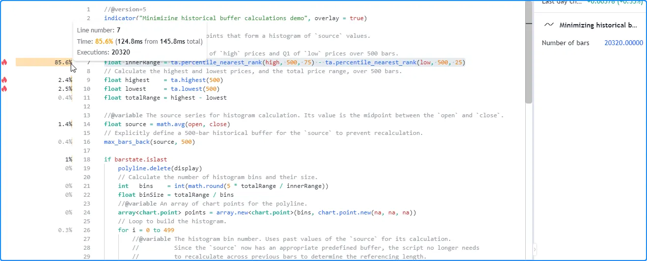
source此脚本将仅引用最后一个历史条和所有实时条上的最近 500 个值。因此,我们可以通过使用max_bars_back()定义 500 条引用长度来帮助它建立正确的缓冲区而无需重新执行
。
在以下脚本版本中,我们在变量声明后添加了max_bars_back(source, 500)
,以明确指定脚本source在执行过程中将访问最多 500 个历史值:
//@version=5
indicator("Minimizing historical buffer calculations demo", overlay = true)

//@variable A polyline with points that form a histogram of `source` values.
var polyline display = na
//@variable The difference Q3 of `high` prices and Q1 of `low` prices over 500 bars.
float innerRange = ta.percentile_nearest_rank(high, 500, 75) - ta.percentile_nearest_rank(low, 500, 25)
// Calculate the highest and lowest prices, and the total price range, over 500 bars.
float highest    = ta.highest(500)
float lowest     = ta.lowest(500)
float totalRange = highest - lowest

//@variable The source series for histogram calculation. Its value is the midpoint between the `open` and `close`.
float source = math.avg(open, close)
// Explicitly define a 500-bar historical buffer for the `source` to prevent recalculation.
max_bars_back(source, 500)

if barstate.islast
    polyline.delete(display)
    // Calculate the number of histogram bins and their size.
    int   bins    = int(math.round(5 * totalRange / innerRange))
    float binSize = totalRange / bins
    //@variable An array of chart points for the polyline.
    array<chart.point> points = array.new<chart.point>(bins, chart.point.new(na, na, na))
    // Loop to build the histogram.
    for i = 0 to 499
        //@variable The histogram bin number. Uses past values of the `source` for its calculation.
        //          Since the `source` now has an appropriate predefined buffer, the script no longer needs
        //          to recalculate across previous bars to determine the referencing length.
        int index = int((source[i] - lowest) / binSize)
        if na(index)
            continue
        chart.point currentPoint = points.get(index)
        if na(currentPoint.index)
            points.set(index, chart.point.from_index(bar_index + 1, (index + 0.5) * binSize + lowest))
            continue
        currentPoint.index += 1
    // Add final points to the `points` array and draw the new `display` polyline.
    points.unshift(chart.point.now(lowest))
    points.push(chart.point.now(highest))
    display := polyline.new(points, closed = true)

plot(bar_index + 1, "Number of bars", display = display.data_window)
经过这一更改,我们的脚本不再需要在所有历史数据中重新执行来确定缓冲区大小。正如我们在 下面的分析结果中看到的那样,全局代码执行的数量现在与图表条的数量一致,并且脚本完成所有历史执行所需的时间大大减少:
注意:
- 此脚本仅需要最近 501 个历史条形图来计算其绘图输出。在这种情况下,优化资源使用的另一种方法是将其包含
calc_bars_count = 501在 indicator() 函数中,该函数通过将脚本可以计算的历史数据限制为 501 个条形图来减少不必要的脚本执行。
提示
解决 Profiler开销问题
由于 Pine Profiler必须执行额外的计算来收集性能数据(如本节所述),因此 在分析时执行脚本所需的时间会增加。
考虑到 Profiler 的开销,大多数脚本都能按预期运行。但是,当复杂脚本的运行时间接近计划 的限制时, 在其上使用Profiler可能会导致其运行时间超出限制。这种情况表明脚本可能需要 优化,但如果无法分析代码,就很难知道从哪里开始 。在这种情况下,最有效的解决方法是减少脚本必须执行的条形图数量。用户可以通过以下任何一种方式实现此减少:
- 选择历史记录中数据点较少的数据集,例如较高的时间范围或数据有限的符号
- 使用条件逻辑将代码执行限制在特定时间或条形范围内
calc_bars_count在脚本的声明语句中包含一个参数,以指定可以使用多少个最近的历史条形图
减少数据点的数量在大多数情况下是有效的,因为它直接减少了脚本必须执行的次数,通常会导致累积运行时间减少。
作为演示,此脚本包含一个gcd()函数,该函数使用
简单算法来计算两个整数的最大公约数。该函数使用两个数字的最小绝对值初始化其。然后,它在while循环中将
result的值减一,
直到它可以将两个数字相除而无余数。此结构要求循环将迭代最多N次,其中N是两个参数中最小的那个。result
在此示例中,脚本绘制了 的值
gcd(10000, 10000 + bar_index)。在本例中,两个参数中最小的一个始终为 10,000,这意味着
函数内的while
循环每次执行脚本将需要最多 10,000 次迭代,具体取决于
bar_index
值:
//@version=5
indicator("Script takes too long while profiling demo")

//@function Calculates the greatest common divisor of `a` and `b` using a naive algorithm.
gcd(int a, int b) =>
    //@variable The greatest common divisor.
    int result = math.max(math.min(math.abs(a), math.abs(b)), 1)
    // Reduce the `result` by 1 until it divides `a` and `b` without remainders.
    while result > 0
        if a % result == 0 and b % result == 0
            break
        result -= 1
    // Return the `result`.
    result

plot(gcd(10000, 10000 + bar_index), "GCD")
当我们将脚本添加到图表中时,它需要一段时间才能在图表数据中执行,但不会引发错误。但是,在 启用 Profiler后,脚本会引发运行时错误,指出它超出了 Premium 计划的运行时间限制(40 秒):
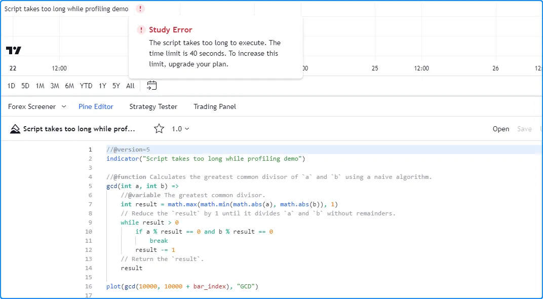
我们当前的图表有超过 20,000 个历史条形图,对于脚本来说,在Profiler处于活动状态时,在规定的时间内处理这些条形图可能太多了 。在这种情况下,我们可以尝试限制历史执行次数来解决此问题。
下面,我们加入了indicator()calc_bars_count = 10000函数
,该函数将脚本的可用历史记录限制为最近的 10,000 个历史条。限制脚本的历史执行后,它在分析时不再超出 Premium 计划的限制,因此我们现在可以检查其性能结果:
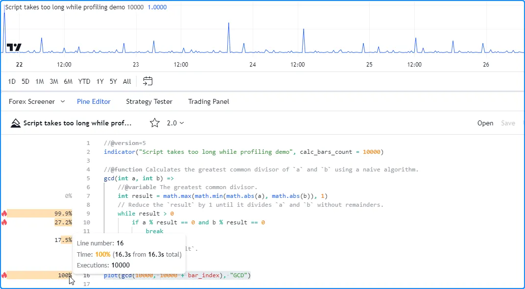
//@version=5
indicator("Script takes too long while profiling demo", calc_bars_count = 10000)

//@function Calculates the greatest common divisor of `a` and `b` using a naive algorithm.
gcd(int a, int b) =>
    //@variable The greatest common divisor.
    int result = math.max(math.min(math.abs(a), math.abs(b)), 1)
    // Reduce the `result` by 1 until it divides `a` and `b` without remainders.
    while result > 0
        if a % result == 0 and b % result == 0
            break
        result -= 1
    // Return the `result`.
    result

plot(gcd(10000, 10000 + bar_index), "GCD")